Easy navigation in LibreOffice Calc. Working with a column Open office how to insert a row

At the request of readers, I publish material on how to fix the table headers so that they do not scroll when viewed, but only the content of the table changes.

We have a table:

Task: fix the header (highlighted in blue in the screenshot) so that when you scroll down the table, it remains in place, and the content scrolls.

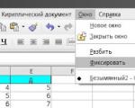
To perform this task, we become in cell A2 and select Window -> Fix

Now when scrolling the table, the title remains in place.

In a similar way, you can freeze a column, or even both a column and a row. To do this, it is important to stand in the cell next to the row and column that you want to fix and mark Fix. For example, to simultaneously fix the first row and the first column, you need to become in cell B2:

To cancel the fix, uncheck the menu item Window -> Fix.

Sometimes a problem arises: to fix, for example, the second column, but so that the first one is not visible. We scroll with a horizontal scroll bar until we have column B on the screen:

We become in cell C1 and achieve the desired result. The main thing then is not to forget that there is also column A, removed from the screen in this way.

A column is a vertical row of cells from row 1 to row 65,536.

How to highlight a column

First way

Second way

2. In the Delete Content window, in the Selection group, select the desired deletion option:

Delete all - to completely delete the contents of the string;

Text - to delete only text (formats, formulas, numbers and dates are not deleted);

Numbers - to delete only numbers (formats and formulas are not deleted);

Date and time - to delete only dates and times (formats, text, numbers and formulas are not deleted);

Formulas - to delete only formulas (text, numbers, formats, dates and times are not deleted);

Notes - to delete only notes to the cells of the row (all other elements are not deleted);

Formats - to remove only the format attributes applied to the cells of the row (the contents of the cells are not deleted);

Objects - to delete only objects (the contents of the cells are not deleted).

3. Close the window with the OK button.

Working with a column A column is a vertical row of cells from row 1 to row 65,536.

How to highlight a column

First way

In the open table window, click on the name of the desired column once with the left mouse button with an arrow cursor.

Second way

In the open table window, select any cell of the required column and use the keyboard shortcut Shift+Ctrl+Space (spacebar).

How to set exact column width

4. In the Column Width window, set the desired value with the Width slider.

The maximum column width is 100 cm.

5. Close the window with the OK button.

How to set the default column width

By default, the column width is considered to be 2.27 cm.

If after changing the width of the columns you want to return to this width, activate the appropriate setting.

1. In the open table window, select the desired column or range of columns.

2. Open the Format menu and in the list of commands, move the cursor over the Column item.

3. In the additional menu, select Width.

4. In the Column Width box, activate the Default option.

5. Close the window with the OK button.

How to hide a column

1. In the open table window, select the desired column or range of columns.

2. Open the Format menu and in the list of commands, move the cursor over the Column item.

3. In the additional menu, select Hide.

Hidden columns will no longer appear, along with their names and the information they contain. This will not break links with hidden cells in formulas and functions.

How to show a range of hidden columns

This method is suitable if the range of hidden columns is known.

1. In the open table window, select the column range that includes the hidden columns.

2. Open the Format menu and in the list of commands, move the cursor over the Column item.

3. In the menu that opens, select Show.

How to show all hidden columns

This method is suitable if the range of hidden columns is unknown or if you want to display all hidden columns.

1. In the open table window, select the entire table field.

2. Open the Format menu and in the list of commands, move the cursor over the Column item.

3. In the additional menu, select Show. How to insert a column

First way

1. In the open table window, select the desired column, to the left of which you want to add a new one.

2. Open the Insert menu.

3. In the command list, select Column.

Second way

1. In the open table window, right-click on the column to the left of which you want to add a new one.

2. In the context menu, select Insert Columns.

To insert multiple columns at the same time, you must first select the desired number of columns.

How to freeze a column on the screen Freezing columns on the screen allows you to work with long rows of data that do not fit in the viewable area of ​​the spreadsheet.

1. In the open table window, select the column to the right of the one that will be fixed, for example, if you need to fix column 10 on the sheet, select column 11.

2. Open the Window menu and select Fix. -All columns to the left of the selected one will be fixed with a non-scrollable area. How to disable column freezing In an open table window, expand the Window menu and disable the Freeze item. How to remove a column

First way

1. In the open table window, select the required column.

2. Open the Edit menu.

3. In the command list, select Delete Cells.

Second way

1. In the open table window, right-click on the desired column.

2. In the context menu, select Delete Columns.

To delete several columns at the same time, you must first select the required number of columns.

How to quickly delete the contents of a column

In the open table window, select the desired column or range of columns and press the Backspace key.

How to selectively clear columns

1. In the open table window, select the desired column or range of columns and press the Delete key.

I think many are already familiar with such a useful tool as Excel, with which you can create a variety of tables for various purposes. Articles with tips about useful tools that can be used in office suites such as Microsoft Office or Libre Office periodically appear on our site.

This guide also belongs to the category of such articles, as examples of how you can freeze rows and columns in Excel from Microsoft or Calc from Libre Office will be shown here, for more convenient viewing of the document.

That is, we will try to make sure that, for example, the first column and the first row are fixed, and the rest of the content of the document can move freely.

How to Freeze Columns or Rows in Microsoft Excel

So, despite the fact that Microsoft Office is a paid office suite, it still remains the most popular among most users who have to deal with documentation, so I think we'll start with Excel.

So, based on the conditions of our example, we need to freeze the first column and the first row.

In this case, left mouse clicks select below the row and column on the right side of the column or row, limiting the fixing area.

That is, if you need to fix the first column and the first row, then you should select the second cell from the row and column, which will be fixed later, for example, in the same way as shown in the screenshot below.

Accordingly, if the task is to fix the first two rows and columns, then we select the third cell, and so on.

In general, in this way we need to show the boundaries of the area that will be fixed in Excel.

Having set the desired border, go to the control panel to the tab " View" - " To fix areas».

Then select " To fix areas».

That's all, after that the rows and columns you need in Excel will be fixed, and you can easily flip through the contents.

I note that there are three items in the area pinning menu:

• To fix areas- is responsible for fixing both columns and rows;
• Pin the top line- by selecting this option you will fix only the first line in your document;
• Freeze first column- Responsible for fixing only the first column.

In general, if you need to fix only one line or column, you can use the second or third paragraph, but if you have several such lines, then you will need to choose the first option.

How to Freeze Columns and Rows in Libre Office Calc

Now for the example in Libre Office Calc. Here, I propose to change the conditions a little and fix the first two lines and the first column.

You can pin them in Calc like this:

As a result, when scrolling the document, the first two lines, as well as the column, will remain in place, but you can easily view all the necessary content of this document.

By the way, in order to return everything to its original state, just go through the same points and select the “Fix rows and columns” option again.

How to Freeze or Freeze Columns and Rows in Excel and LibreOffice Calc

At the request of readers, I publish material on how to fix the table headers so that they do not scroll when viewed, but only the content of the table changes.

We have a table:

Task: fix the header (highlighted in blue in the screenshot) so that when you scroll down the table, it remains in place, and the content scrolls.

To perform this task, we become in cell A2 and select Window -> Fix

Now when scrolling the table, the title remains in place.

In a similar way, you can freeze a column, or even both a column and a row. To do this, it is important to stand in the cell next to the row and column that you want to fix and mark Fix. For example, to simultaneously fix the first row and the first column, you need to become in cell B2:

To cancel the fix, uncheck the menu item Window -> Fix.

Sometimes a problem arises: to fix, for example, the second column, but so that the first one is not visible. We scroll with a horizontal scroll bar until we have column B on the screen:

We become in cell C1 and achieve the desired result. The main thing then is not to forget that there is also column A, removed from the screen in this way.

single cell

Left click on a cell. The result will be as shown in Fig. 5 on the left. You can make sure that the selection is correct in the Sheet area field.

Range of adjacent cells

A range of adjacent cells can be selected using the keyboard or mouse. To select a range of cells by moving the mouse cursor:

Select nonadjacent cells

A range of nonadjacent cells can be selected using the Ctrl + mouse key:

Working with columns and rows

Insert columns and rows

Columns and rows can be inserted in several different ways in an unlimited number.

Individual column or row

1. Do either Insert > Columns or Insert > Rows.

When inserting one new column, it is inserted to the left of the selected column. When inserting one new line, it is inserted above the selected line.

An individual column or row can also be inserted using the mouse:

1. Select the column or row where you want to insert a new column or new row.
2. Click on the title with the right mouse button.
3. Do either Insert > Columns or Insert > Rows.

Multiple columns or rows

Multiple columns or rows can be inserted at once rather than one at a time.

1. Select the required number of columns or rows and, holding down the left mouse button on the first of them, move the cursor to the required number of headings.
2. Proceed as you would when inserting one column or one row as above.

Removing columns and rows

Columns and rows can be deleted individually or as a group.

Individual column or row

One column or row can only be deleted with the mouse:

1. Select the column or row to be removed.
2. Right-click on a column or row header.
3. Execute from context menu Remove columns or Delete lines.

Multiple columns or rows

Multiple columns or rows can be deleted at once instead of being deleted one at a time.

1. Select the desired number of columns or rows by holding down the left mouse button on the first one and drag the cursor over the desired number of headings.
2. Proceed as you would when deleting one column or row as above.

Work with sheets

Like any other Calc element, sheets can be inserted, deleted, and renamed.

Inserting new sheets

There are many ways to insert a new sheet. The first step in all methods is to select sheets, after which a new sheet will be inserted. After that, you can use the following steps.

• Open the Insert menu and select Sheet, or
• Right-click on the tab and select Add Sheets, or
• Click on the empty space at the end of the row of sheet tabs (Fig. 9).

Each method leads to the opening of the Insert Sheet dialog box (Fig. 10). In it, you can determine whether the new sheet will be placed before or after the selected sheet, as well as how many sheets to insert.

Deleting Sheets

Sheets can be deleted individually or as a group.

Separate sheet

Right-click on the tab of the sheet to be deleted and select Delete from the context menu.

Multiple sheets

To delete several sheets, select them as described above, right-click on any tab and select Delete from the context menu.

Renaming sheets

The default name for a new sheet is "Sheet X", where X is a number. This works well when there are only a few sheets for a small spreadsheet, but becomes inconvenient when there are a large number of sheets. To give a sheet a more meaningful name, you can:

• When creating a sheet, enter your name in the Name field, or
• Right-click on the sheet tab and select Rename and replace the existing name with the new one from the context menu.

Sheet names must begin with either a letter or a number; other characters, including spaces, are not allowed, although spaces can be used between words. Attempting to rename a sheet with an incorrect name results in an error message.

Appearance Calc

Fixing Rows and Columns

A fix locks the top few rows, or the few columns on the left side of the sheet, or both. When scrolling within a sheet, any frozen rows and columns remain within the author's view.

On fig. 11 shows fixed rows and columns. A thickened horizontal line between rows 3 and 16, as well as a thickened vertical line between columns C and H, separate the fixed areas. Rows 4 to 16 and columns D to G are scrolled up. The fixed three rows and three columns remained in place.

The fix point can be set after one row, one column, or after both, as shown in Figure 2. eleven.

Freeze individual rows or columns

• Click on the heading below the fixed row or to the left of the fixed column.
• Execute the command Window > Lock.

A dark line will appear, indicating the boundary of the fixation.

Row and column fixation

• Select the cell located immediately after the fixed row and immediately to the right of the fixed column.
• Execute the command Window > Lock.

Two lines will appear on the screen, horizontal above this cell and vertical to the left of this cell. Now, when scrolling, all lines above and to the left of these lines will remain in place.

Deleting a commit

To remove the fixation of rows or columns, run the command Window > Lock. The checkbox next to Fix should disappear.

Window split

Another way to change the look is to split the window - also known as split screen. The screen can be split either horizontally or vertically, or both. This allows you to view up to four sheet fragments at any time.

What is it for? Imagine that you have a large worksheet and in one of its cells there is a number used in three formulas in other cells. Using split screen, you can arrange a cell containing a number in one section, and each of the cells with formulas in other sections. Then you can change the number in the cell and see how it affects the contents of cells with formulas.

Split screen horizontally

To split the screen horizontally:

1. Place the mouse cursor on the vertical scroll bar on the right side of the screen and position the cursor over the small arrow button at the top.

1. A thick black line is visible directly above this button (Figure 13). Move the mouse cursor to this line; as a result, the cursor will change its shape to a line with two arrows (Fig. 14).

1. Hold down the left mouse button, a gray line will appear across the page. Drag the cursor down, the line will follow the cursor.
2. Release the mouse button and the screen will split into two images, each with its own vertical scroll bar.

On fig. 11, the values ​​"Beta" and "A0" are located at the top of the window, and other calculation results are at the bottom. The top and bottom parts can be scrolled independently. Therefore, you can change the values ​​of Beta and A0, observing their influence on the results of calculations in the lower half of the window.

It is also possible to split the window vertically, as discussed below - the results are the same, allowing both sides of the window to be scrolled independently. Having vertical and horizontal separation, we get four independent windows for scrolling.

Split screen vertically

To split the screen vertically:

1. Place the mouse cursor on the horizontal scroll bar at the bottom of the screen and position the cursor over the small arrow button on the right.

1. A thick black line is visible directly to the right of this button (Figure 15). Move the mouse cursor over this line, as a result the cursor will change its shape to a line with two arrows.
2. Hold down the left mouse button, a gray line will appear across the page. Drag the cursor to the left, the line will follow the cursor.
3. Release the mouse button and the screen will split into two images, each with its own horizontal scroll bar.

You can also split the screen using the same procedures as for fixing rows and columns. Follow these directions, but instead of doing Window > Lock, use Window > Split.

Entering data into a sheet

Entering numbers

Select a cell and enter a number in it using the top row of the keyboard or the numeric keypad.

To enter a negative number, enter a minus sign (–) in front of the number, or enclose it in parentheses ().

By default, numbers are right-justified, and negative numbers have a minus sign in front of them.

Entering text

Select a cell and enter text in it. Text is left-aligned by default.

Entering numbers as text

If the number is entered in the format 01481, Calc will remove the leading 0. To keep this leading zero, in the case of entering codes, for example, prefix the number with an apostrophe, like: "01481. However, the data is now treated as text by Calc. Arithmetic operations will not work. The number will either be ignored or an error message will appear.

Numbers can have leading zeros and are treated as text if the cell is formatted appropriately. Right click on a cell and select Cell Format > Number. Setting the value to Leading Zeros allows you to have numbers with leading zeros.

Even if you declare a variable as text, it can still participate in arithmetic operations; however, the result of such operations may differ from what is expected. In some cases, Calc will perform arithmetic on a cell that contains text, whether it has characters (such as ABCD) or numbers that you have formatted as text. For more information, see the Calc Guide.

Entering date and time

Select a cell and enter the date and time in it. Date elements can be separated from each other by a (/) or (-) symbol, or you can use text such as 10 Oct 03. Calc recognizes many date formats. Time elements can be separated by a colon, such as 10:43:45.

Autocomplete

The Autofill mode allows you to facilitate and speed up data entry - a fill marker in the form of a black square in the lower right corner of the current cell (it works, in addition to entering formulas, with numbers, dates, days of the week, months and mixed data).

Automated data entry:

1. 1.In the first cell of the range, enter the value of one of the list items;
2. 2. move the mouse cursor over the fill marker so that it takes the form of a cross;
3. 3.drag the fill marker, highlighting the range (if the selected range is greater than the number of elements in the list, then it will be filled cyclically).

If you enter two consecutive numbers into two adjacent cells that make up the beginning of an arithmetic progression, for example, 1 and 3, then select them and, as when copying, use the fill handle to drag them over several cells, the series will continue: 1, 3, 5, 7 etc. If you need to fill in the cells with a step of one, then just enter the first number, for example 1, and use the fill marker to drag it to the desired number, we get a series of 1, 2, 3, etc.

Org Calc also allows you to enter non-numeric sequences. For example, if you enter January into a cell and perform the operation described above, then February, March, etc. will appear in the following cells.

Leave your comment!