How to change number value in excel. The cell format is not changed. To change the font color

The cell format includes parameters that determine: » the type of representation of the numeric value of the cell; » cell content alignment and orientation; » type of font; « cell framing; filling (background) of the cell. In addition, you can set the protection settings for the data written to the cell. Cells are usually formatted by changing individual

parameters. Before you can change the format of a cell, you must place a table cursor on it. If you want to set the format for several cells at the same time, you must first select these cells.

Standard Formats Excel has six standard cell formats (sets of options) that can be used in all documents. When you start a new spreadsheet, all cells have the same default standard format. This format is called Normal. It has the following options:

The depicted value repeats the true value;

Horizontal alignment depends on the type of data;

Vertical alignment is performed on the bottom edge;

Text without word wrap;

The displayed value orientation is horizontal;

Content is displayed in a standard font without highlights or effects;

There is no border around the cells;

There is no filling.

The rest of the standard formats differ from the Normal format only by displaying numbers in cells:

Financial (or Separated) - the number is rounded to two decimal places, for example, the number 43.569 is represented as 43.57;

Financial(0) - the number is rounded to the nearest integer, for example, the number 43.569 is represented as 44;

Monetary - the number is rounded to two digits after the decimal separator and a currency sign is added, for example, the number 43.569 on a "Russian" computer is represented as 43.57 rubles;

Monetary (0) - the number is rounded off as a whole and a currency sign is added, for example, the number 43.569 is represented as 44 rubles;

Percentage - if a number from 0 to 1 is entered into the cell after setting the format, then it is multiplied by 100, then the number (regardless of the value) is rounded to an integer and a% sign is added to it, as a result of this, for example, the numbers 0.43569 and 43.569 will be presented equally 44%. If in the Options dialog box, on the Edit tab, turn off the Automatic input, percent switch, then all numbers will be multiplied by 100, and not just from 0 to 1. As a result of this, for example, the numbers 0.43569 and 43.569 will be represented as 44% and 4357 %. The same will happen if this switch is enabled, but the numbers were entered into the cells before they were assigned the Percentage format.

When using financial and currency formats, the separator between the digits of units, thousands, millions, etc. is set in the Windows settings: the Numbers tab in the Language and Standards program in the Control Panel. This is usually a space. When setting up Windows, the sign of the currency unit is also set: the Currency tab in the Language and Standards program in the Control Panel. For the ruble, this is usually r. The thousands separator used can be changed without changing the general Windows setting.

To do this, in the Options dialog box, on the International tab, in the Numbers group, turn off the Use system separators switch and enter a different separator in the Digit separator field. Sometimes a comma or an apostrophe is used as such a separator. To apply standard formats, the corresponding tools of the Formatting panel and keyboard shortcuts, as well as the Style dialog box, can be used. Representation of a numeric value As already noted, the values ​​after they are entered into the cells have the form set by default.

However, it is possible to change the appearance of the cells as you wish. You can use the Formatting toolbar and keyboard shortcuts to change individual settings. However, the Format Cells dialog box provides the most complete cell formatting options. To call the Format Cells window, do one of the following:

Run command Cells...(Format);

Execute the Format Cells... command from the context menu of a cell (selected cells);

Press the combination Ctrl + 1.

On the Number tab of the Cell Format window, the Number formats list contains the names of the groups of representations of numeric values ​​available in Excel. By default, the list is set to General, which displays numeric values ​​as entered by the user. After selecting another value, additional options appear on the tab, with the help of which the parameters for the appearance of numerical values ​​are set.

For example, when you select Numeric, the following appears:

Field Number of decimal places - setting the number of characters after the decimal separator;

Thousands separator switch - enable the digits separator (space) between groups of digits of units, thousands, millions, etc.;

List Negative numbers - selection of the type of representation of negative numbers. When choosing a format, it is convenient to use the Sample field, which changes in accordance with changes in the tab options. If the value (all formats) is selected in the Number formats list, then the Type list appears, which includes all available number formats, which, however, are written in the form of codes (conventional symbols). Having dealt with these codes, the user in the Type field can independently set the formats.

So, for example, the following notation is used in format codes:

An optional digit, i.e. if there is no digit in place of the # sign in the number, then nothing is displayed in this place;

Mandatory digit, i.e. if there is no digit in place of the 0 sign, then zero is displayed in this place (usually, the output of zeros after the decimal separator is set in this way, for example, the format 0.000 sets the mandatory display of three characters after the separator);

Mandatory place, i.e. if in place of the sign? there is no digit in the number, then a space is displayed in this place (usually this ensures the alignment of numbers in one column, for example, the format ?????0.00 sets the alignment to the decimal separator of all numbers that have up to six digits before the separator); h, hh, m, mm, s, ee, D, DD hours, minutes, seconds and days of the month h:m will look like 6:7, and in the format hh:mm - 06:07); M, MM, MMM, MMMM month (for example, February in different formats will look like 2.02, fairy, February); IT, YYYY year (recorded using 2 or 4 digits, respectively).

Separators in date and time formats are determined by the settings specified in the Windows settings:

the Date and Time tabs in the Language and Standards program in the Control Panel. For more information about the conventions used in codes, see the Excel help system. The user-created format can then be deleted by clicking the Delete button. When changing the format of numerical values, their true values ​​(entered or calculated by formulas) do not change, i.e., for example, no matter how many decimal places are displayed, all available characters will be used in formula calculations.

In other words, setting a new format only changes the appearance of the numeric value, not changing its value. At the same time, it is possible to set such a mode in which the accuracy of the true values ​​will always be equal to the accuracy of the representation of numbers on the screen. To do this, in the Options dialog box, on the Calculations tab, in the Book Options group, turn on the screen accuracy switch. This setting will apply to all tables in the book.

To set the format of numerical values, the Formatting panel can be used, on which the following tools are located:

Monetary Format Set the standard format to Monetary;

Percent Format Set the default format to Percentage;

Delimited Format Sets the standard format Financial,

Increase bit depth increase by one the number of characters after the decimal separator;

Decrease bit depth..;

decrease by one the number of characters after the decimal separator. Keyboard shortcuts for setting numeric value formats:

Ctrl+Shift+" .... set the format to Normal;

CtrI+Shift+1 ... set the number format to 0.00 with a separator of groups of digits;

Ctrl+Shift+2.... set time format to hmm;

Ctrl+Shift+Z.... set the date format to DD. MMM.YY;

Ctrl+Shift+4.... set the format to Monetary;

Ctrl+Shift+5.... set format Percentage;

CtrI+Shift+6.... setting the format to 0.00E+00 (exponential view). If a numeric value is entered in a cell, but you want it to be perceived by the program as text, then for such a conversion in the Cell Shape dialog box on the Number tab, in the Number formats list, select the Text value.

A useful and often overlooked feature in Excel is finding (and changing) the formatting of cell content. For example, for cell data that uses the 14-point Calibri font, it's easy to specify a different font and font size. However, this process isn't as intuitive as it could be, so I'll walk you through it step by step.

Let's assume that the contents of most of the worksheet cells use a yellow background and a 14-point Calibri bold font. In addition, the same cells are available on other sheets of the workbook. Let's change the formatting of the contents of all these cells as follows: font - Cambria; style - bold; size - 16 points; the color of the letters is white; cell color - black.

To change formatting using Find and Replace, follow these steps:

1. Select any cell (or multiple cells if you want to search within a specific range) and select the command Home Editing Find and Select Replace(or click ctrl+h) to display the window Find and Replace.
2. Make sure the Find and Replace fields on the Find and Replace dialog box are empty.
3. Click the button Format next to the field To find to open the dialog Find Format. If this button is not visible, click the button Options.
4. In the dialog box Find Format you can specify formatting options. But to speed up this procedure, click on the arrow next to the button Format, select a command Select format from cell, and then click the cell with the formatting you want to replace.
5. Now press the button Format next to the field Replace on to display the dialog box Replace Format.
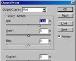
6. And again: either choose a command Select format from cell and specify the cell with the content whose formatting you want to replace, or use the tabs of the dialog box Replace Format to specify the desired formatting. Go to the tab Font and select Cambria, set the size to 16, bold, and set the text color to white. On the tab fill select black as the background color of the cell. If you have set the same settings, then your Find and Replace dialog box should look like the one in Figure 1. 22.1.
7. Click the Replace All button.

Using the command in step 4 Select format from cell, you may find that the content formatting is not replaced in all cells. The fact is that, as a rule, one or more formatting settings do not match. For example, you will not be able to apply formatting to the contents of a cell that is set to a number format. General, to the contents of a cell that has a number format the date. To fix this, click the button Format and then in the dialog box To find format on each tab that does not match the settings you specified, click the Clear button.

In some cases. for example, you want to write about how to buy a furniture tour to China, a visa to China, tickets to China, then it’s better to just select cells of a certain format. To do this, follow steps 1 to 4 and then click the button Find all. The dialog box will show more information about the matching cells.

Click on the list at the bottom of the dialog box, and then press the keyboard shortcut Ctrl+A. Now that all matching cells are selected, you can format them however you like. Note that by dragging the column borders, you can increase their width, as well as sort the contents of a column by clicking on its header.

Unfortunately, Excel 2010 never provided the ability to search for cells by their styles using the Find and Replace dialog box. While Microsoft (since Excel 2007) has put a lot of emphasis on cell styles, there is no way to find all cells that use a particular style and apply a different style to those cells. You can find and replace formatting, but the cell style will not change.

Changing the cell format in Excel allows you to organize the data on a sheet into a logical and consistent chain for professional work. On the other hand, incorrect formatting can lead to serious errors.

The contents of a cell is one thing, but the way the contents of the cells are displayed on the monitor or printed is another. Before you change the data format in an Excel cell, you should remember a simple rule: "Everything that the cell contains can be presented in different ways, and the presentation of the data display depends on the formatting." This is easy to understand if shown with an example. See how you can use formatting to display the number 2 in different ways:

Most Excel users use only standard formatting tools:

• buttons on the Home panel;
• ready-made cell format templates available in the dialog box are opened using the CTRL + 1 hot key combination.

Data formats entered into spreadsheet cells

Fill in the cell range A2:A7 with the number 2 and format all cells as shown in the figure above.

The solution of the problem:

What options does the Format Cells dialog box provide? The functions of all the formatting tools that the Home tab contains can be found in this dialog box (CTRL+1) and even more.

In cell A5, we used the financial format, but there is also a monetary format, they are very often confused. The two formats differ in the way they are displayed:

• the financial format, when displaying numbers less than 0, puts a minus on the left side of the cell, and the money format puts a minus in front of the number;
• the default currency format displays negative values ​​in red font (for example, enter the value -2p in the cell and the currency format will be assigned automatically);
• in financial format, 1 space is added after currency reduction when displaying values.

If you press the hotkey combination: CTRL + SHIFT + 4, then the cell will be assigned the monetary format.

As for the date in cell A6, it's worth mentioning the Excel rules here. The date format is considered as a sequence of days from January 1, 1900. That is, if the cell contains a value - the number 2, then this number in the date format should be displayed as 01/02/1900 and so on.

Time for Excel is the value of numbers after the decimal point. Since we have an integer in cell A7, the time is displayed there accordingly.



Date format with time in Excel

Let's format the data table so that the values ​​in the rows are displayed according to the column names:

In the first column, the formats already correspond to its name, so go to the second and select the range B3:B7. Then press CTRL + 1 and on the "Number" tab, specify the time, and in the "Type:" section, select the display method as shown in the figure:

We do the same with the ranges C3:C7 and D3:D7, choosing the appropriate formats and display types.

If the cell contains a value greater than 0 but less than 1, then the date format in the third column will be displayed as: January 0, 1900. While in the fourth column the date is already displayed differently due to a different type (1904 date systems, see below for details). And if the number

Notice how the time is displayed in cells that contain fractional numbers.

Since dates and times in Excel are numbers, it is easy to perform mathematical operations with them, but we will consider this in the next lessons.

Two Excel date display systems

There are two systems for displaying dates in Excel:

1. The date January 1, 1900 corresponds to the number 1.
2. The date January 1, 1904 corresponds to the number 0, and 1 is already 01/02/1904, respectively.

Note. In order for all dates to be displayed by default according to the 1904 system, you can make the appropriate settings in the parameters: “File” - “Options” - “Advanced” - “When recalculating this book:” - “Use the 1904 date system”.

We clearly give an example of the difference in the display of dates in these two systems in the figure:

The Excel help lists the minimum and maximum numbers for dates in both systems.

The settings for changing the date system apply not only to a specific sheet, but to the entire program. Therefore, if there is no urgent need to change them, then it is better to use the default system - 1900. This will avoid serious errors when performing mathematical operations with dates and times.

Unformatted spreadsheets can be hard to read. Formatted text and cells can draw attention to certain parts of the spreadsheet, making them visually more visible and easier to understand.

There are many text and cell formatting tools in Excel. In this lesson, you'll learn how to change the color and style of text and cells, align text, and set a custom format for numbers and dates.

Text formatting

Many text formatting commands can be found in the Font, Alignment, Number groups on the ribbon. Group commands Font allow you to change the style, size, and color of the text. You can also use them to add borders and fill cells with color. Group commands alignment allow you to set the display of text in the cell both vertically and horizontally. Group commands Number allow you to change how numbers and dates are displayed.

To change the font:

1. Select the desired cells.
2. Click the drop-down arrow for the font command on the Home tab. A dropdown menu will appear.
3. Hover your mouse over different fonts. The selected cells will interactively change the font of the text.
4. Choose the font you want.

To change the font size:

1. Select the desired cells.
2. Click the drop-down arrow for the font size command on the Home tab. A dropdown menu will appear.
3. Hover your mouse over different font sizes. The selected cells will interactively change the font size.
4. Choose the font size you want.

You can also use the Increase Size and Decrease Size commands to change the font size.

To use bold, italic, underline commands:

1. Select the desired cells.
2. Click on the command bold (W), italics (K) or underlined (H) in the Font group on the Home tab.

To add borders:

1. Select the desired cells.
2. Click on the command dropdown arrow borders on the home tab. A dropdown menu will appear.
3. Select the desired border style.

You can draw borders and change line styles and colors using the border drawing tools at the bottom of the dropdown menu.

To change the font color:

1. Select the desired cells.
2. Click the drop-down arrow next to the Text Color command on the Home tab. The Text Color menu appears.
3. Hover your mouse over different colors. The sheet will interactively change the text color of the selected cells.
4. Choose the color you want.

The choice of colors is not limited to the drop-down menu. Select More Colors at the bottom of the list to access an expanded Color selection.

To add a fill color:

1. Select the desired cells.
2. Click the drop-down arrow next to the Fill Color command on the Home tab. The Color menu appears.
3. Hover your mouse over different colors. The sheet will interactively change the fill color of the selected cells.
4. Choose the color you want.

To change the horizontal alignment of text:

1. Select the desired cells.
2. Select one of the horizontal alignment options on the Home tab.

• Align text to the left: Aligns text to the left of the cell.
• Align Center: Aligns text to the center of the cell.
• Align text to the right: Aligns text to the right of the cell.

To change the vertical alignment of text:

1. Select the desired cells.
2. Select one of the vertical alignment options on the Home tab.

• Top edge: Aligns text to the top of the cell.
• Align in the middle: Aligns text to the center of the cell between the top and bottom edges.
• Along the bottom edge: Aligns text to the bottom of the cell.

By default, numbers align to the right and bottom of the cell, while words and letters align to the left and bottom.

Formatting numbers and dates

One of the most useful features of Excel is the ability to format numbers and dates in many different ways. For example, you may want to display numbers with a decimal separator, a currency or percentage symbol, and so on.

To set the format for numbers and dates:

Numeric Formats

1. General is the default format of any cell. When you enter a number in a cell, Excel will suggest the number format that it thinks best. For example, if you enter "1-5", the cell will display a number in the Short Date format, "1/5/2010".
2. Numerical formats numbers to decimal places. For example, if you enter "4" in a cell, the number "4.00" will be displayed in the cell.
3. Monetary formats numbers in display form currency symbol. For example, if you enter "4" into a cell, the number will be displayed as "" in the cell.
4. Financial formats numbers similar to the Currency format, but additionally aligns currency symbols and decimal places in columns. This format will make long financial lists easier to read.
5. Short date format formats numbers as M/D/YYYY. For example, the entry August 8, 2010 would be represented as "8/8/2010".
6. Long date format formats numbers as Day of Week, Month DD, YYYY. For example, "Monday, August 01, 2010".
7. Time formats numbers as HH/MM/SS and signed AM or PM. For example, "10:25:00 AM".
8. Percentage formats numbers to decimal places and a percent sign. For example, if you enter "0.75" into a cell, it will display "75.00%".
9. Fractional formats numbers as fractions with a slash. For example, if you enter "1/4" into a cell, the cell will display "1/4". If you enter "1/4" into a cell with the General format, the cell will display "4-Jan".
10. Exponential formats numbers in scientific notation. For example, if you enter "140000" into a cell, the cell will display "1.40E+05". Note that by default, Excel will use exponential format for a cell if it contains a very large integer. If you don't want this format, then use Number Format.
11. Text formats numbers as text, that is, everything in the cell will be displayed exactly as you entered it. Excel uses this format by default for cells that contain both numbers and text.
12. You can easily customize any format using Other Number Formats. For example, you can change the US dollar sign to another currency symbol, change the display of commas in numbers, change the number of decimal places to display, and so on.