home › Wallpaper › Features of data entry and editing. Editing and formatting data in cells of Excel worksheets 1 data entry in microsoft excel

Features of data entry and editing. Editing and formatting data in cells of Excel worksheets 1 data entry in microsoft excel

Excel allows you to enter three types of data into cells: numbers, text, formulas. Text can be used for table headings, explanations, or notes on a worksheet. If Excel does not recognize the data type as numeric or as a formula, then the data is treated as text.

Numbers are used to represent digital information and can be entered in a variety of formats: general, monetary, financial, percentage, and so on. Date and time can also be thought of as numbers.

Formulas entered into a cell perform calculations, control the operation of the database, check the properties and values of cells, and are used to establish the relationship between cells and arrays using address links.

Any formula begins with a (=) sign. If a formula is entered in a cell, then by default the cell will show the calculation result.

Entering data into a cell

The data is typed directly in the active cell, while they are displayed in the formula bar. Also, data can be typed in the formula bar.

Data input

Click in a cell.
Enter data like 2001 Annual Report.
Press the key Enter.
To cancel your entry, press Esc.

As you type in the formula bar, click the button Enter- √ to confirm, and to cancel the entry press the button Cancel - ×.

Pressing the arrow keys or clicking on another cell Will always cause the typed data to be saved in the active cell before moving to the next.

Text that is too wide to fit into the current cell will visually overlap with adjacent cells, when in fact it will be contained in one cell. Excel limits text or formulas in a cell to 255 characters.

Numbers that are too large to be shown inside the current cell will be displayed as a sequence of characters # # # #. To show a numeric value in a cell, you need to increase the column width (see the section "Formatting cells").

You can delete the contents of the cell using the key Delete.

Selecting cells

Many operations, such as inserting rows or columns, deleting, copying or moving cells, require one or more cells to be selected before starting the operation.

The selection area can be either a separate cell or take up an entire workbook. The active cell is always part of the selection. The selection area must be rectangular and can be defined as:

one or more cells;
one or more columns;
one or more lines;
one or more worksheets.

Tab. 17 illustrates some of the possible combinations.

Table 17. Designations of table areas

Cells can be selected using the mouse or keyboard, or a combination of both (Table 18). Selected cells will be different in color.

Selection area	Allocation method
Single cell	Click in a cell
Cell group	Click, with the mouse in the cell; without releasing the mouse, drag from the first cell to the last, or click the first cell and hold down the Shift key and click the last cell
Column	Click on the column heading
Adjacent columns	Click on the first column heading; without releasing the mouse, drag from the first column header to the last, or click on the first column header and hold down the Shift key and click on the last column header
Line	Click on the row header
Adjacent lines	Click on the row header; without releasing the mouse, drag from the first row heading to the last, or click on the first row heading and hold down the Shift key and click on the last row heading
All cells in the current worksheet	Click on the button at the intersection of the row and column headings
Discontiguous columns	Select the first column, press Ctrl and select the following columns
Non-contiguous lines.	Select the first line, press Ctrl and select the following lines
Non-contiguous cells	Select the first group of cells, press Ctrl and select the next group of cells

Table 18. Selection of table areas

Click on any cell to deselect it. To select an area with the mouse, if the selection area exceeds the size of the window, as in other applications, auto-scrolling is used. This means that if the mouse pointer goes beyond the borders of the window, the sheet will automatically scroll in that direction.

Editing cell contents

Editing the contents of a cell can be done either in the cell or in the formula bar. The Input and Edit modes are shown in the status bar.

To edit, double-click in the cell you want to edit, or click in the formula bar.

The mouse pointer can be used to move to the edit location. In addition, the following keys can be used in edit mode:

Just like in Word, pressing the Insert key toggles between insert and overwrite modes.

Undo and redo actions

Excel allows you to undo changes made to a workbook. Although this function is applicable to the majority commands, there are exceptions for it (for example, you cannot undo the deletion and renaming of a sheet).

Command Undo on the Edit menu context sensitive. When the user types or edits data in the formula bar, the menu Edit the command corresponding to the last performed operation will be offered.

On the standard panel to undo the last commands press the button or cancel several commands by selecting them from the list.

After choosing a team Undo in the Edit menu the command will change to the Redo command.

Insert Rows and Columns

Additional rows or columns can be inserted as needed anywhere in the table. Command Insert on the Edit menu can be used to insert a new column left from the current column or new row above the current line.

Multiple columns and rows can be added by selecting an area that includes more than one column or row.

Select as many columns or rows as you want to insert.
Please select Insert, Rows or Insert, Columns or press the key combination Ctrl and + on the numeric keypad.

To remove rows or columns:

Select the rows or columns to remove.
Please select Edit, Delete or press the key combination Ctrl and - on the numeric keypad.

When inserting and deleting columns or rows, the addresses of the remaining data in the table are shifted, so you need to be especially careful when inserting or deleting.

Moving and copying data

Moving and copying data is one of the main operations used when working with tabular data, while not only the contents of the cells are copied to a new place, but also their formatting.

Moving and copying the contents of cells can be done in two ways:

using the Edit menu commands;
dragging with the mouse.

As soon as the user selects a cell and selects the command Cut or Copy (Cut or Soru) on the menu Edit Excel will copy the contents of the cell to the clipboard.

When you move, the data of the original cells will be pasted to the new location.

Data copying is used to duplicate information. Once the content of one cell is copied, it can be pasted into a separate cell or into a region of cells multiple times. In addition, the selected area is surrounded by a movable dashed border, which will remain until the operation is completed or canceled.

The border looks like a pulsating dotted box that surrounds the selected object. Inserting the contents of cells is only possible when this border exists.

Using the command Paste on the Edit menu after choosing the Cut command will cut off the border.

Using the command Paste after the Copy command will not disable the border i.e. the user can continue to specify other insertion destinations and use the command Insert again.

Keystroke Enter will paste the selection at the new location indicated by the mouse and turn off the border.

Keystroke Esc will undo the copy to clipboard operation and disable the border.

When inserting data from more than one cell, you only need to specify the upper left corner of the area of cells on the worksheet into which you are inserting.

Moving and copying using the menu

Possibility Drag and Drop allows you to move or copy the contents of the selected cells using the mouse. This feature is especially useful when moving and copying over short distances (within the visible area of the worksheet).

Drag and drop move and copy

Select the area of cells to move.
Move the mouse pointer over the selection border.
Use the pointer to drag the selection to a new location. The cell area will be moved to a new location.
If you hold down the key while dragging Ctrl, the cell area will be copied to the new location.

Special data copy

Special copying of data between files includes the command Special Paste Special on the Edit menu (Edit). Unlike the usual copying of data using the Paste command, the command can be used to calculate and transform information, as well as to link workbook data (these possibilities will be discussed in the next chapter).

Command Piste Special often used to copy the formatting attributes of a cell.

Select the cell or cells to copy.
Select the cell or cells where the source data will be placed.
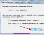
Please select Edit, Paste Special. The Paste Special dialog box contains several options for pasting data (Figure 83).

Rice. 83. Paste Special

Set the necessary parameters, for example, formats (when collocating formats, only the formatting is changed, not the value of the cells).
Please select OK.

The first group of dialog box options Paste Special allows you to select the content or formatting attributes you want to insert. Selecting the All (AI) option pastes the content and attributes of each copied cell to a new location. Other options allow you to insert different combinations of content and / or attributes.

The second group of parameters is used only when inserting formulas or values and describes the operations performed on the information being inserted into cells that already contain data (Table 19).

Parameter	Insertion Result
To fold	The inserted information will add up to the existing values
Subtract	The inserted information will be subtracted from the existing values
Multiply	The existing values will be multiplied by the inserted information
Divide	The existing values will be divided by the inserted information
Skip blank cells	You can perform actions only for cells containing information, that is, with special copying, empty cells will not destroy existing data
Transpose	The orientation of the pasted area will switch from rows to columns and vice versa

Table 19. Parameters of the Paste Special command

Choice No (None) means that the copied information simply replaces the contents of the cells. Choosing other options for operations, we get that the current content will be merged with the inserted information and the result of such merging will be the new contents of the cells.

The exercise

Performing Calculations Using Paste Special

Enter the data as shown in table. twenty.

	A	V	WITH	D	E	F	G	N
1
2	5	2					1	2
3	12	3					10	3
4	8	2					15	4

Table 20. Initial data

Select the area to copy A2: A4.
Choose Edit, Copy.
Click cell B2 (the upper left corner of the area where the data will be placed).
Choose Edit, Paste Special.
Set the Multiply option.
Click on OK. Notice that the border of the selection area remains on the screen.
Click cell C2, which will be the start of the insertion area.
Please select Edit, Paste Special, and set the Transpose option.
Copy the formats of column G yourself to column H and get a table. 21.

	A	B	C	D	E	F	G	N
1
2	5	10	5	12	8		1	2
3	12	36					10	3
4	8	16					15	4

Table 21. Result of the Paste Special command

Data input

The current cell is highlighted with a gray border called a cell selector. Moving around the worksheet is carried out using the cursor keys: [arrows], , , or by clicking on any other cell.

You can enter into a cell:

text- the text is aligned to the left border of the cell;

the numbers- numbers are aligned on the right border of the cell;

formulas- the first character of the formula is the "=" sign, then the cell addresses and arithmetic operations follow.

Confirmation of input carried out:

key ;

by clicking in another cell;

Refusal to enter carried out:

key ;

by clicking a button in the formula bar.

Correcting cell contents

To correct when filling the cell, before the text input is confirmed, it is possible to use the key ... If you need to correct the already confirmed content of the cell, then you need to do double click with the mouse on this cell. In this case, a flashing vertical line will appear in the cell - text cursor, which will allow you to correct the data in the cell.

Removing the contents of a cell

If you need to delete the contents of a cell, just set the cell selector to this cell and press the key .

Formatting data

Formatting data in a cell refers to the formatting of the contents of a cell or a block of cells in various modes.

The main modes for designing worksheets are collected in a team Format - Cells ... The dialog that appears contains row of tabs to select a mode:

Number:

In the dialog on the right, there is a list of formats containing the following formats: Numerical; Monetary; Date; Text etc.

Alignment:

The dialog that appears contains three groups of modes: Horizontal; Vertical; Orientation... Each mode has a number of mutually exclusive parameters. In addition, there is a switch Wrap by words, with its help, you can fill a cell with text in several lines, and inside one cell.

Font:

In the dialog that appears, there are fields with the name of the font, style and size, as well as some effects.

Frame:

First, you need to select the block in which the frames are drawn. The dialog contains two groups of modes that allow you to select the style and color of the line, as well as the position of the line relative to the selected block.

View:

On this tab, select the fill and pattern of the selected cells.

Editing
data

Insertion and deletion

To insert new cell, you need to select a cell, front which should be inserted another one, and select the menu command Insert - Cells ...(data shifted to the right or shifted down).

If you need to insert column cells, then select the column, front with which a new one should be inserted, and select the menu command Insert - Column or Insert - Cells ...(column). In this case, the format of the cells of the inserted column will be the same as the cells of the selected column.

To insert strings the line is highlighted, above which will insert the new one. Select team Insert - Rows or Insert - Cells ...(line). Accordingly, the inserted lines take the format of the selected ones.

Delete an entire column, row or cell can be done using the menu command True - Delete ...

Copy and move

Moving and copying is based on usage Clipboard... Copying is done using the menu commands - Edit - Copy and Insert... Command copy the selected block is copied to clipboard. Further
when using the command Insert content buffers can be copied anywhere in the document. Team work Cut similar to team work Copy with the only difference that the team Cut removes the selected text from the document and transfers it to buffer
exchange. On the toolbar Standard there are three corresponding buttons.

Similarly, using the mouse, you can move Cell Content: The mouse pointer over the cell selector frame has the shape of its normal arrow. While holding down the left mouse button, drag the frame to a new location. You can move both the contents of one cell and the contents of a block of cells. With the key pressed the contents of the cell will be copied.

Copy to adjacent cells

In addition, it is possible to copy to adjacent cells using the mouse: the cell selector in the lower right corner has a thickening in the form of a black square. The mouse pointer at this point changes to a black plus sign. Now, while holding down the left mouse button, drag the frame to adjacent cells. You can drag the frame only horizontally or vertically.

Assignment 2

Develop a business letter template in a Microsoft Word word processor.

Business letter

————————————————————————————————————————————————-

Assignment 3

Develop in a spreadsheet processor Microsoft Excel - Summary of changes in the amounts of deposits in three branches of the bank by days of one week.

Table 1 - Summary of changes in the amounts of deposits in three branches of the bank by days of one week

Full name date of completion
Bank's name	Contribution name	Interest rate	Deposit amount	Summary of changes in deposit amounts by day of one week
Bank's name	Contribution name	Interest rate	Deposit amount
Bank 1	Pension	8,50%	15000	15003,5	15007	15010,5	15014	15017,5	15021	15024,5
	Egg capsule	10,25%	15000	15004,2	15008,4	15012,6	15016,9	15021,1	15025,3	15029,5
	Agro-Hit	11,30%	15000	15004,6	15009,3	15013,9	15018,6	15023,2	15027,9	15032,5
Bank 2	Premium	10,00%	15000	15004,1	15008,2	15012,3	15016,4	15020,6	15024,7	15028,8
	Savings	7,50%	15000	15003,1	15006,2	15009,2	15012,3	15015,4	15018,5	15021,6
	Confidant	13,75%	15000	15005,7	15011,3	15017	15022,6	15028,3	15033,9	15039,6
Bank 3	Travel	11,25%	15000	15004,6	15009,2	15013,9	15018,5	15023,1	15027,8	15032,4
	Money box	13,00%	15000	15005,3	15010,7	15016	15021,4	15026,7	15032,1	15037,4
	Anniversary	12,00%	15000	15004,9	15009,9	15014,8

ENTERING AND EDITING DATA IN MICROSOFT EXCEL

1. Data entry

All data that is entered into a Microsoft Excel spreadsheet is placed and stored in cells. Each cell can hold up to 255 characters. Excel uses two types of data: constants and formulas. Constants include text, numeric values, including date and time, which, when typed, are displayed in the table cell and in the input area of the formula bar (Fig. 1). Moreover, one cell can contain either a number or text, but not a number and text together. Formulas set the calculation algorithm, the results of which are displayed in cells, and the formula itself, by which the result is calculated, is in the input area of the formula bar (Fig. 2).

Rice. 1. Constant in a table cell.

Rice. 2. Displaying the formula in the table.

To enter data into a cell, you must select it, and then start entering by pressing the necessary characters on the keyboard. Moreover, the input of decimal fractions is carried out with a "comma" sign between the integer and fractional parts of the number.

Data can be entered directly into a cell in a worksheet or into the input area of a formula bar. In this case, the information entered is displayed simultaneously in these two places. To complete the entry of data into a cell, do one of the following:

1) press the Enter or Tab keys;

2) click on the button for entering the formula bar;

3) press one of the cursor keys.

By default, Microsoft Excel sets all table columns to the same width. Therefore, when entering large numbers and long text, the last characters either "disappear" (if the adjacent cell is full) (cell B13 in Fig. 3), or "crawl" onto the adjacent cell (if it is empty) (cell E6 in Fig. 3). But at the same time, the entered data is in the cell and is fully displayed in the formula bar. In such cases, you should change the column width (row height) automatically or manually.

In addition, a cell may display ##### data if it contains a number that does not fit in the column. To see this number, you need to increase the column width.

Rice. 3. Display of "long" data in the table.

To automatically resize a column, place the mouse pointer on the right border of the column heading so that it looks like a cross with a double-headed arrow, and double-click the left mouse button.

To change the column width (row height) manually, place the mouse pointer on the right border of the column header (lower border of the row header) so that it looks like a cross with a double-headed arrow (Fig. 4) and, while holding down the left mouse button, drag the right border the column heading (bottom border of the row heading) in the new position.

Rice. 4. Changing the column width manually.

In this case, the tooltip will display

set column width. It shows the average number of digits 0-9 in the default font that fits in the cell, and the column width in pixels.)

In order to change the width of several columns at once, select the columns whose width you want to change, and then drag the right border of the header of any selected column. Similarly, you can change the height of several lines at once.

2. Faster data entry

V Microsoft Excel can make data entry easier by using the AutoComplete, Select From List, and AutoComplete tools, and by using a fill handle.

The AutoComplete tool completes text input for the user. As you enter characters in a cell, AutoComplete checks all cells in the column from the current cell to the first blank cell. If

it will find in the column a data element starting with the entered characters, then the remaining characters will be entered automatically according to the found pattern.

Suppose a column contains a sequence of text data, for example, city names: Kiev, Chisinau, Kislovodsk. The first two letters are the same. When you enter the first three letters Kish into a new cell in a column, the AutoComplete tool will insert the word Kishinev (Figure 5). If you need to enter another word, then you need to continue entering the remaining characters. If you need to enter exactly the word Chisinau, you need to press Enter. The AutoComplete tool makes it very easy to enter large amounts of text data, especially in cases where the differences in words start with the second or third letter.

Rice. 5. Tool Completion.

AutoComplete does not work with numeric values.

The Select from List tool is used if the user knows that the required text has already been entered in one of the cells in this column. To do this, just right-click on the active cell and select Select from the drop-down list from the context menu. A list will open under the active cell, in which all text data entered into this column will be presented (Fig. 6). The user must left-click on the list item that needs to be placed in the active cell.

Rice. 5. Tool Selection from the list.

The Select from List tool, like the AutoComplete tool, works

only the contents of the column cells are not separated by blank cells and does not work with numeric values.

To fill cells in a row or column with duplicate values, you can use filling with fill marker ( black square in the lower right corner of cell_ (fig. 7).

Rice. 7. Fill marker.

To do this, follow these steps:

1) enter into the cell the value that you want to fill in the row or column;

2) select this cell again;

3) move the mouse pointer to the fill handle so that the mouse pointer changes to a black cross;

4) while holding down the left mouse button, drag the pointer, which has taken the form of a cross, over the required cells of the row (column) (Fig. 8).

To fill the cells of a row or a column with a sequence of numbers, in which each next number differs from the previous one by the same value (by an arithmetic progression), you can:

1) enter the value of the first member of the arithmetic progression into the cell;

2) enter the second member of the arithmetic progression into the adjacent cell of the row or column;

3) select both cells;

4) holding the left mouse button, drag the fill handle to the right (if you need to fill the row cells) or down (if you need to fill the column cells) (Fig. 9)

Rice. 9. Filling the cells of the column with arithmetic progression values using the fill marker.

Also, to set the progression, you can use the Fill Groups Editing button on the Home tab and in the Progression dialog box that appears, set the parameters for the arithmetic or geometric progression.

Microsoft Excel allows you to enter frequently repeating lists into a table using the AutoComplete tool. After installation, Microsoft Excel already contains lists of days of the week and months. In some of them, their elements are complete words, and in others, generally accepted abbreviations:

- January, February, March,…, December;

- Jan, Feb, Mar,…, Dec;

- Monday, Tuesday, Wednesday,…, Sunday

Mon, Tue, Wed,…, Sun

To automatically enter one of these lists, you should:

1) enter the first element of the list into the cell;

2) select this cell;

3) keeping the left mouse button pressed, drag the fill handle to the right or down (fig. 10).

Rice. 10. Tool Autocomplete.

If you need to use your own, non-built-in lists, then the user can assign them to autocomplete. This requires:

3) in the Lists dialog box that opens, in the Lists field, select the New list item;

4) click in the List items field and enter your list, using the Enter key to separate the list items (Fig. 11);

5) after specifying the last element of the list, click on the Ok button.

Rice. 11. Create your own autocomplete list.

A new autocomplete list can also be created based on the already entered

v list of values table:

1) select a range of cells containing a list;

2) on the Office Button menu, click the Excel Options button;

3) in the Excel Options dialog box that opens, in the General section, click the Edit Lists button;

4) in the Lists dialog box that opens, click the Import button.

5) click on the Ok button.

Rice. 12. Creation of the autocomplete list based on the list of values already entered in the table.

3. Editing data

Data entered into a cell in Microsoft Excel can be edited right as you enter it. Editing of already entered data can be done in two ways - directly in the cell (for this you need to go to edit mode) or using the input area of the formula bar. To enter edit mode, you can either double-click the cell or press the F2 key. To edit data using the formula bar, you must select the cell and click once in the input area of the formula bar. Editing data in a cell is similar to editing text in Microsoft Word. To delete the character located to the left of the cursor, use the Backspace key, and to delete the character located to the right of the cursor, use Delete. When you enter and

Data is always entered into the active cell with a green border. When you start Excel for the first time, cell A1 is active by default (Fig. 3.1). To activate another cell, you need to place a selection frame on it. This can be done by clicking on it with the mouse button or by moving the frame to the desired cell using the cursor keys. After selecting a cell, type a text, number or formula in it (entering complex formulas using built-in Excel functions will be discussed in a separate paragraph).

The simplest example of a table created in Excel is shown below in Fig. 3.2.

Rice. 3.1.

Rice. 3.2.

Use a comma when entering decimal fractions. Excel treats numbers containing a period, hyphen, or slash as dates. So, if you type 1.5, 1/5 or 1-5 in cell, the system recognizes this entry as the first of May of the current year, transforming it into 01 May. The full date (in the format "DD.MM.EEEE" - 05/01/2013) can be seen in the formula bar by highlighting

cell. To enter a date containing a different year, type sequentially, separated by a period, hyphen or slash, day, month and year. The colon is used to enter the time. So, if you type 3:15 in cell, Excel recognizes that record as 3:15:00.

Press Enter to finish typing and move to the next lower cell, or press Tab to move to the cell to the right of the current cell, or use the mouse or cursor keys to move to other cells.

If the width of the entered text exceeds the width of the cell, it will be superimposed on the empty cells on the right, but will not fill them. If there is data in the cells on the right, then the typed text will not intersect with them. When you remove the selection frame from a cell, the text will be "clipped" to the width, but you can see it in full in the formula bar by "clicking" on the cell. However, there is an easy way to get rid of the overlap - change the width of the column with this cell. To do this, move the mouse pointer over the right border of the column heading and, when it turns into a double-headed arrow, press the left mouse button and drag the border to the right until all the text is displayed. This is how the width of the first column in Fig. 3.2. To set the exact width of the column, watch the value in the tooltip while dragging the border. To change the width of a column automatically to the longest content of the cell in that column, simply double-click the right border of the column header.

You can also render text that does not fit in the width of the cell in another way - word wrap by increasing the line height. Select the required cell by clicking the mouse button and on the tab home in a group Alignment press the button Transfer text Ш 1 Transfer text. In this case, the height of the row in which the cell is located will be increased so that its hidden content is fully displayed. To wrap text according to words, the cell height can also be changed manually: by dragging it beyond the border of the header, as in the case of a column.

To enter simple formulas containing only arithmetic signs (+, -, *, /), follow these steps:

select by clicking the cell where you want to place the formula;
enter the equal sign = (this should always be done when typing formulas);
enter the addresses of the cells, the values of which will take part in the calculation. To do this, click on the first one. In this case, the cell will be highlighted with a running frame, its address will appear in the input cell (Fig. 3.3);
type an arithmetic sign from the keyboard (multiplication is indicated by an asterisk - *, division with a slash - /, and exponentiation with a circumflex sign - L) and click to select the second cell to insert its address (Fig. 3.3) or type the address from the keyboard, switching to English layout;
press Enter on your keyboard to complete your input.

As a result, the cell will display the result of the calculation.

Rice. 3.3.

You can combine several arithmetic operations in one formula. Use parentheses if necessary, as with standard notation for mathematical expressions. For example, if you need to add the values of two cells, then divide the result by the number in the third cell, in the form of a formula it will look like this: = (B2 + C2) / D2. When entering a formula, specify cell addresses by clicking or typing manually.

To delete the contents of a cell, select it by clicking it and press the Delete key; if you need to type new data in a filled cell, it is not necessary to delete the previous one - just select it and start entering. The old data will be automatically replaced.

A cell can contain a large piece of text or a complex formula, which cannot be completely removed to make changes. You should double-click on the cell, position the cursor in the desired place for editing, or click in the formula bar in the required part of the arithmetic expression, make the necessary changes and press the Enter key.

You can refuse to edit a cell, even if you have already started doing it. To do this, just press the Esc key. This will restore the original data in the cell. To cancel an action already taken, press the standard Ctrl + Z key combination or the button Cancel on Quick access panels.

When you change the values in the cells referenced by the formula, the result of the calculations in the cell containing the formula will be automatically recalculated.

Auto-completion. Often, when filling out a table, you have to type the same text. The auto-completion function available in Excel helps to significantly speed up this process: if the system determines that the typed part of the text coincides with the one that was entered earlier in another cell, it will substitute the missing part and highlight it in gray (Figure 3.4).

Rice. 3.4.

You can agree with the proposed option and proceed to filling in the next cell by pressing the key Enter , or continue typing the desired text, ignoring the selection when the first few letters match.

Autocomplete. The autocomplete mechanism is useful when you need to enter any sequence of data into cells.

Autocomplete can be used when entering times, dates, days of the week, months, and combinations of text with a number. To do this, you only need to enter the first value. Excel will determine the principle of filling in the remaining cells on its own, increasing the current value by one (Fig. 3.5). If you need to enter the same values at a certain interval, proceed as described above by entering the first two values so that Excel can determine the difference between them.

When working with cells, it is important to separate the concepts of "cell content" and "cell format". Content is the entered data. The format includes not only the formatting applied to the cell (content alignment, data font settings, fill, border), but also the data format in the case when the cells contain numbers. We will talk about number formats and cell formatting techniques below, but now we will consider the issue of copying formats using autocomplete.

In order to use the autocomplete feature, place the mouse cursor on the lower right corner of the cell so that the cursor takes the form of a black "cross", then press the left mouse button and without releasing it, move the cursor in the desired direction (you can copy down, up, right and left).

With this method of autocomplete with numbers, dates and times, Excel performs an arithmetic progression (increasing or decreasing the original value by several units). And to make a geometric progression, you need to press and hold the right mouse button, after selecting the desired range of cells, a context menu will open in which select the item Progression... and in the dialog box select the type of progression geometric and also specify a step or check the box Automatic detection of hiaga.

Suppose you formatted a cell, set a specific number format, and want to extend the format of this cell to a number of others without pasting content. To do this, select a cell and perform an autofill operation by dragging the frame beyond the lower marker. After you release the mouse button, the button will appear in the lower right corner of the row. T * Autocomplete options. By clicking on it, you will open a menu in which you can select the method of filling the cells (Fig. 3.6).

Rice. 3.5.

with different types of autocomplete data

In this case, to copy the format, select the item Fill in formats only.

If you want to apply autocomplete only to the contents of cells without preserving the format, run the command Fill in values only. By default, the contents of the cells are copied (with the creation of a sequence if possible) and their format.

1. Entering data into Excel cells

Data is always entered into the active cell with a black border. When you start Excel for the first time, cell A1 is active by default. To activate another cell, you need to place a selection frame on it. This can be done by left-clicking or moving the frame to the desired cell using the cursor keys.

After selecting a cell, you need to type text, number or formula in it.

Numeric values can contain numbers from 0 before 9 , as well as special characters: + - E e ()., $% /

To enter a numerical value in a cell, you must select the desired cell and enter the required combination of numbers from the keyboard. The numbers you enter appear both in the cell and in the formula bar. Upon completion of the entry, press the Enter key. After that, the number will be written into the cell. By default, after pressing Enter, the cell located one row below becomes active, but using the "Service" - "Options" command, you can set the required direction of transition to the next cell after entering, or exclude the transition altogether on the "Edit" tab. If, after entering a number, press any of the cell navigation keys (Tab, Shift + Tab ...), the number will be fixed in the cell, and the input focus will go to the adjacent cell.

The peculiarities of entering numeric values using special characters are as follows.

1. If you need to enter a negative number, then the number must be preceded by a "-" (minus) sign.

2. Symbol E or e used to represent a number in exponential notation. For example, 5e3 means 5 * 1000, i.e. 5000.

3. Numbers in parentheses are interpreted as negative, even if there is no minus sign in front of the number. Those. (40) - for Excel means -40.

4. When entering large numbers for convenience of representation between the groups of digits, you can enter a space (23 456.00). In this case, the space in the formula bar will not be displayed, and in the cell itself, the number will be with a space.

5. The dollar sign ($) is used to enter the currency format.

6. Use the percent sign (%) to enter the percentage format.

7. Use the forward slash (/) to enter dates and fractional values. If Excel can interpret the value as a date, for example 1/01, then the cell will represent the date - January 1. If you need to represent such a number as a fraction, then you must enter zero - 0 1/01 before the fraction. A fraction will also represent a number that cannot be interpreted as a date, for example 88/32.

Sometimes it becomes necessary to enter long numbers. At the same time, to display it in the formula bar, an exponential notation with no more than 15 significant digits is used. The precision of the value is chosen such that the number can be displayed in the cell.

In this case, the value in the cell is called the input or display value.

The value in the formula bar is called the stored value.

The number of digits entered depends on the column width. If the width is not wide enough, Excel either rounds the value or prints ### characters. In this case, you can try increasing the cell size.

When entering decimal fractions, you must use a comma. Excel treats numbers containing a period, hyphen, or slash as dates. So, if you type in cell 1.5, 1/5 or 1-5, the system recognizes this record as the first of May of the current year, transforming it into 01 May. The full date (in the format day. Month. Year - 05/01/2007) can be seen in the formula bar by selecting the cell.

If you need to enter a date containing another year, you need to type consecutively through a period, hyphen or slash the number, month and year, for example, 7.8.99, 25/6/0, or 12–12–4. As a result, Excel will place the dates 08/07/1999, 06/25/2000 and 12/12/2004 in the cells. The colon is used to enter the time. So, if you type 19:15 in cell, Excel recognizes that record as 19:15:00. To complete typing and move to the next bottom cell, you must press the Enter key, or use the mouse or cursor keys to move to other cells.

If the text you enter is wider than the width of the cell, it will overlap, but not fill, empty cells on the right. If there is data in the cells on the right, then the typed text will not overlap with them. When you remove the selection frame from the cell, the text will be "clipped" in width, but you can see it in full in the formula bar by clicking on the cell. However, there is an easy way to get rid of the overlap by changing the width of the “bad” cell column. To do this, move the mouse pointer over the right border of the column header and when it becomes

, click and drag the border to the right until all the text is displayed. To set the exact width of a column, watch the value on the tooltip while dragging the border. An even easier way to set the desired width is to double-click on the border of the column header.

You can also render text that does not fit in the width of the cell in another way - word wrap by increasing the line height. To do this, select the problem cell by clicking and on the Home tab, in the Alignment group, click the Text Wrap button

... In this case, the height of the row in which the cell is located will be increased so that its hidden content is fully displayed. To wrap text, according to words, the cell height can be changed manually by dragging the header beyond the border, as in the case of a column.

To enter simple formulas containing only arithmetic signs (+, -, *, /), you need to do the following:

1. Select the cell where you want to place the formula by clicking.

2. Enter the equal sign = (this should always be done when typing formulas).

3. Next, you need to enter the addresses of the cells, the values of which will take part in the calculation. To do this, you need to click on the first of them. In this case, the cell will be highlighted with a running frame, and its address will appear in the input cell (Fig. 1, left).

4. After that, type an arithmetic sign from the keyboard and click to select the second cell to insert its address (Fig. 4, right) or type the address from the keyboard, switching to the English layout. Next Press Enter to complete the entry. As a result, the result of the calculation will be displayed in the cells.

5. It is possible to combine several arithmetic operations in one formula. If necessary, you can use parentheses, as in the case of standard notation of mathematical expressions. So, for example, if you need to add the values of two cells, and then divide the result by the number in the third cell, in the form of a formula it will look like this: = (B2 + C2) / D2. When entering a formula, cell addresses must be clicked or typed manually.

Rice. 1 - Entering the simplest formula

2. Editing data in a cell

Editing of data in a cell is carried out as follows. To delete all the contents of a cell, click to select it and press the key. If you need to type new data in a filled cell, it is not necessary to delete the previous one. Just highlight it and start typing. The old data will be automatically replaced.

If a cell contains a large text fragment or a complex formula, then it is completely irrational to delete them to make changes. Double-click on the cell, place the cursor in the desired place for editing, make the necessary changes and press Enter.

If you need to refuse to edit a cell, but editing has already begun, just press the Esc key. This will restore the original data in the cell. To undo an action already taken, use the standard keyboard shortcut + Z or the Undo button on the Quick Access Toolbar.

When you change the values in the cells referenced by the formula, the result of the calculations in the cell containing the formula will be automatically recalculated.

3. Autocomplete and autocomplete cells

Often, when filling out a table, you have to type the same text. Excel's AutoComplete feature helps speed up this process significantly. If the system determines that the typed part of the text coincides with what was entered earlier in another cell, it will substitute the missing part and highlight it in black (Fig. 2). You can agree with the proposal and proceed to filling in the next cell by clicking, or continue typing the desired text, not paying attention to the selection (if the first few letters match).

Rice. 2 - Autocomplete when entering text

The autocomplete mechanism is useful when you need to enter a sequence of data into cells. Suppose you need to fill a row or column with a sequence of numbers, each of which is greater (or less) than the previous one by a certain amount. In order not to do this manually, you can do the following:

1. It is necessary to type in two adjacent cells the first two values from a series of numbers so that Excel can determine their difference.

2. Select both cells.

3. Move the mouse pointer over the marker located in the lower right corner of the selection frame. At the same time, it will take the form of a black plus.

4. Click and, while holding down the mouse button, drag the frame until the final value appears on the tooltip near the mouse pointer, which will be placed in the last cell of the row. You can drag the frame in any direction.

5. Release the mouse button to fill the range of covered cells.

The autocomplete feature is very useful when copying a formula across a series of cells. Thanks to the autocomplete feature, you can enter formulas into cells in a matter of seconds. You need to type only the first formula, and then drag the frame over the lower marker to copy it to the entire row.

Popular in the heading: