Descriptive statistics based on the Excel Data Analysis Pack. Two-way analysis of variance with repetitions
This article will discuss how to analyze data using a pivot table. For training you can use the table available at this link (simple table.xlsx).
The first thing that might need to be analyzed with a pivot table is to summarize the subtotals. In our example, it may be necessary to calculate the sales volumes for all stores for each date.
To do this, you need to click on any header of the pivot table row (in our example, these are the fields Date, Point of Sale and Phone Brand), and in the opened tabs Working with pivot tables go to tab Options... It is necessary to press the button on it. Field parameters in a group Active field.
In the window that opens, the first tab will be a bookmark.
The absence of such a tab means that you have not selected the row header, that is, the cursor is positioned on a cell with a numeric value.
On a bookmark Subtotals and Filters You can select a condition for subtotal output. The following conditions are offered:
- automatically - calculates the amount for each condition in the table;
- no - subtotals are not calculated;
- others - allows you to independently select an action for summing up subtotals.
By setting automatic subtotals, we get the following table, which contains the subtotals for each condition:

If setting up subtotals using the command Field parameters, does not give visible results, check the settings for displaying subtotals using the command Subtotals group Layout tabs Constructor.
Let's say we want to display subtotals for dates only, hiding the subtotals for POS. To do this, click on any field of the table with the store name and call the context menu. In it, you need to uncheck the condition Subtotal: Point of Sale... As we can see, subtotals are left only for dates:

It is often necessary to sort the data of the pivot table for better perception. To do this, just select the field by which you want to sort, go to the tab General, in a group Editing push the button Sort and filter and set the sorting conditions you need.
A very useful feature for analyzing information in a pivot table is the ability to group data. For example, we need to group our sales by week of the month. To do this, you need to select the dates that are included in the first week (15.05-21.05):

Please note that for ease of selection, we collapsed the data for individual stores by using the + button on the left side of the cell with the store name.
Next, you need to run the command Grouping by selection group Group tabs Options... A new column appears in the table, in which the field Group1 will combine the fields we selected.

All that remains is to rename the group name by simply editing the cell:

To cancel grouping, just use the command Ungroup from the same group, having previously selected the field to be ungrouped. Please note that you cannot ungroup a field that we included in the condition for building a PivotTable - for example, the field Point of sale or date.
Let's consider another way of displaying data that will help us analyze information from our table. For example, we need to know the volume of revenue not in monetary terms, but as a percentage of the total revenue for the entire sales period.
To do this, you need to select any cell in the Revenue column of our pivot table. After that, you need to run the command Field parameters in a group Active field tabs Options.

In the dialog box that opens, go to the tab Additional calculations and from the drop-down menu select the item Percentage of total by column... After clicking the OK button, our table will look like this:

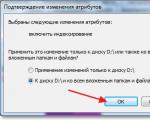
If the data in the table will not be displayed as percentages, check the settings for the number format of the cells (this can be done immediately in the dialog box Field parameters by pressing the button Number format, or by calling the corresponding window from the context menu).
If you need to develop complex statistical or engineering analyzes, you can save steps and time with an analysis package. You provide data and parameters for each analysis, and the tool uses the appropriate statistical or engineering functions to calculate and display the results in an output table. Some tools create charts in addition to the output tables.
Data analysis functions can only be applied on one sheet. If the data analysis is carried out in a group consisting of several sheets, then the results will be displayed on the first sheet, on the remaining sheets empty ranges containing only formats will be displayed. To analyze the data on all sheets, repeat the procedure for each sheet separately.
Note: To enable a Visual Basic for Applications (VBA) feature for an analysis package, you can download the add-in " Analysis Package - VBA"in the same way as when loading an analysis package. Available add-ins check the box Analysis Package - VBA .
To download an analysis pack in Excel for Mac, follow these steps:
If the add-in Analysis package is not in the field list Available add-ons, press the button Overview to find her.
If a message appears stating that the analysis package is not installed on your computer, click Yes to install it.
Exit Excel and restart it.
Now in the tab Data command available Data analysis.
On the menu Service select add-ons Excel.
In the window Available add-ons check the box Analysis package and then click OK.
I cannot find an analysis package in Excel for Mac 2011
There are several third-party add-ins that provide Analysis Pack functionality for Excel 2011.
Option 1. Download the KSLSTAT add-in statistical software for Mac and use it in Excel 2011. KSLSTAT contains over 200 basic and advanced statistical tools that include all the features of the analysis suite.
Select the version of KSLSTAT that matches your Mac OS and download it.
Open the Excel file that contains the data and click the XLSTAT icon to open the XLSTAT toolbar.
Within 30 days you will have access to all KSLSTAT functions. After 30 days, you can use the free version, which includes the functions of the analysis package, or order one of the more complete KSLSTAT solutions.
Option 2. Download Statplus: Mac LE for free from Analystsoft and then use Statplus: Mac LE with Excel 2011.
You can use Statplus: Mac LE to perform many of the functions that were previously available in analysis packages, such as regression, histograms, variance analysis (Two-way ANOVA), and t-tests.
Go to the analystsoft website and follow the instructions on the download page.
After downloading and installing Statplus: Mac LE, open the workbook containing the data you want to analyze.
Microsoft Excel is one of the most irreplaceable software products. Excel has such broad functionality that, without exaggeration, it can be used in absolutely any area. With the skills in this program, you can easily solve a very wide range of problems. Microsoft Excel is often used for engineering or statistical analysis. The program provides the ability to set a special setting, which will greatly help to facilitate the task and save time. In this article, we'll talk about how to enable data analysis in Excel, what it includes, and how to use it. Let's get started. Go!
To get started, you need to activate an additional analysis package
The first thing to start with is to install the add-on. We will consider the whole process using the example of Microsoft Excel 2010. This is done as follows. Go to the File tab and click Options, then select the Add-Ins section. Next, find "Excel Add-ins" and click on the "Go" button. In the window of available add-ons that opens, select the "Analysis package" item and confirm your choice by clicking "OK". If the required item is not in the list, you will have to find it manually using the "Browse" button.

Since Visual Basic functions may still be useful to you, it is advisable to install the "VBA Analysis Pack" as well. This is done in a similar way, the only difference is that you have to select another add-in from the list. If you know for sure that you don't need Visual Basic, then you don't need to download anything else.

The installation process for the Excel 2013 version is exactly the same. For the 2007 version of the program, the only difference is that instead of the "File" menu, you must click the Microsoft Office button, then follow the steps as described for Excel 2010. Also, before starting the download, make sure that the latest version of NET is installed on your computer. Framework.
Now let's look at the structure of the installed package. It includes several tools that you can apply depending on your tasks. The list below contains the main analysis tools included in the package:

As you can see, using the data analysis add-in in Microsoft Excel gives you much broader possibilities of working in the program, making it easier for the user to perform a number of tasks. Write in the comments if the article was useful for you and if you have any questions, be sure to ask them.
TASK number 1
Statistical data analysis in MS Excel
Purpose of work: to learn how to process statistical data using built-in MS Excel functions; explore the capabilities of the Analysis Package and its tools: “ Generating random numbers ", "Bar graph" , " Descriptive statistics " on the example of processing measurements of the speed of movement.
In accordance with the guidelines for the laboratory work "Measuring the speed of vehicles" (in the discipline "Search and design of highways"), process the experimental measurement data by methods of mathematical statistics in Excel. For what:
1. Calculate statistical characteristics using the built-in functions: - the minimum value of the movement speed Vmin;
The maximum value of the speed of movement Vmax; - the average value of the speed of movement Vav;
Standard deviation S;
Standard deviation of the mean Sav;
Student's coefficient (to determine the confidence interval) t; - confidence interval for P = 0.95.
2. Get statistical characteristics using the tool "Descriptive statistics"From the additional package" Data Analysis ".
3. Construct a histogram of the movement speed distribution.
4. Build a cumulative curve (cumulative frequency curve).
5. Construct a theoretical curve of the distribution of the speed of movement.
To obtain a sufficient amount of initial data (speed measurement results), use a simulation experiment using the tool " Generating random numbers»Add-on« Data Analysis ».
When performing p.p. 3 and 4 to select the interval of speeds ("pocket" - in Excel terminology), allowing to obtain the most symmetric histogram showing the normal distribution law.
An example of execution is given in the attached file BasicsPK1-Student.xls.
Methodical instructions
Suppose that we have performed a series of 10 experiments, measuring a certain value of X. Table 1. Approximate view of the "Processing experiment" sheet
The entries in columns D and E are hints that will help you figure out what characteristics we will calculate. Column F should be empty for now, our formulas will be placed in it.
We start processing the results by calculating the number of experiments n.
To determine the number of values, a special function called COUNT is used. To enter a formula with functions, use the Function Wizard, which is launched by the "Insert Function" command through the "Insert" - "Function" menu or by the button on the toolbar with the designation f x.
Let's click on cell F6, where the result should be located and launch the Function Wizard.

The first step of work (Figure 1) serves to select the desired function.
Statistical functions are used to process experimental data. Therefore, first of all, in the list of categories, select the "Statistical" category. A list of statistical functions appears in the second window.
The list of functions is sorted alphabetically, which makes it easy to find the COUNT function we need ("Counts the number of numbers in the list of arguments").
Having selected this function by clicking, press the Ok button and go to step 2.
The second step (Figure 2) is used to set the arguments to the function.
The COUNT function needs to indicate which numbers it needs to recalculate, or in which cells these numbers are located. The next two stages of processing a series of experiments are carried out in a similar way.
In cell F7, using the AVERAGE function, the average value of the sample is calculated, in cell F8, the standard deviation of the sample, using the STDEV function. ...
The arguments of these functions are all the same range of cells.
To calculate the confidence interval, it is necessary to determine the Student's coefficient. It depends on the probability of error (with a generally set reliability of 95%, the probability of error is 5%), and on the number of degrees of freedom n-1).
To find the Student's coefficient, use the Excel statistical function TYUDRASPONV (“Student's distribution is inverse”). A feature of this function is that the first argument, the number 5% (or 0.05), is entered into the corresponding window from the keyboard. For the second, specify the address of the cell where the value of n is, then add “-1” in the window. We get the record “F6-1”.
The usual multiplication formula is used to find the confidence interval. Of course, instead of letters, there should be the addresses of the cells where the Student's coefficient and the standard deviation of the mean are located. As a rule, the value of the confidence interval is rounded to one significant digit, the same order of the environment should be in the mean. Therefore, the final result can be written as follows: with 95% reliability X = 14.80 ± 0.05. In conclusion, let's calculate the relative error in determining X: = CI / X cf (formula: “= F11 / F7”). The value of the relative error is usually expressed as a percentage, we have 0.3%.
To perform tasks 2 and 3, the "Analysis package" add-in is used (from the menu Tools Data Analysis Histogram).
To install an add-on, open the Tools Add-ons menu and select "Analysis package" from the list of available add-ons available for installation (see. Installing add-ons
Excel on computer.doc).