How to solve simple integrals. Online calculator. Calculate the indefinite integral (antiderivative). Historical background for the emergence of the concept of integral
If the definitions from the textbook are too complex and unclear, read our article. We will try to explain as simply as possible, “on the fingers”, the main points of such a branch of mathematics as definite integrals. How to calculate the integral, read in this manual.
From a geometric point of view, the integral of a function is the area of the figure formed by the graph of a given function and the axis within the limits of integration. Write down the integral, analyze the function under the integral: if the integrand can be simplified (reduced, factored into the integral sign, divided into two simple integrals), do so.


To test yourself or at least understand the process of solving an integral problem, it is convenient to use the online service for finding integrals, but before you start solving, read the rules for entering functions. Its greatest advantage is that the entire solution to the problem with an integral is described here step by step.
Of course, only the simplest versions of integrals are considered here - certain ones; in fact, there are a great many varieties of integrals; they are studied in the course of higher mathematics, mathematical analysis and differential equations in universities for students of technical specialties. A function F(x) differentiable in a given interval X is called antiderivative of the function
f(x), or the integral of f(x), if for every x ∈X the following equality holds:
F " (x) = f(x). (8.1) Finding all antiderivatives for a given function is called its integration. Indefinite integral function
f(x) on a given interval X is the set of all antiderivative functions for the function f(x); designation -
If F(x) is some antiderivative for the function f(x), then ∫ f(x)dx = F(x) + C, (8.2)
Table of integrals
Directly from the definition we obtain the main properties of the indefinite integral and a list of tabular integrals:
1) d∫f(x)dx=f(x)
2)∫df(x)=f(x)+C
3) ∫af(x)dx=a∫f(x)dx (a=const)
4) ∫(f(x)+g(x))dx = ∫f(x)dx+∫g(x)dx
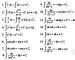
List of tabular integrals
1. ∫x m dx = x m+1 /(m + 1) +C; (m ≠ -1)
3.∫a x dx = a x /ln a + C (a>0, a ≠1)
4.∫e x dx = e x + C
5.∫sin x dx = cosx + C
6.∫cos x dx = - sin x + C
7. = arctan x + C
8. = arcsin x + C
10. = - ctg x + C
Variable replacement
To integrate many functions, use the variable replacement method or substitutions, allowing you to reduce integrals to tabular form.
If the function f(z) is continuous on [α,β], the function z =g(x) has a continuous derivative and α ≤ g(x) ≤ β, then
∫ f(g(x)) g " (x) dx = ∫f(z)dz, (8.3)
Moreover, after integration on the right side, the substitution z=g(x) should be made.
To prove it, it is enough to write the original integral in the form:
∫ f(g(x)) g " (x) dx = ∫ f(g(x)) dg(x).
For example:
Method of integration by parts
Let u = f(x) and v = g(x) be functions that have continuous . Then, according to the work,
d(uv))= udv + vdu or udv = d(uv) - vdu.
For the expression d(uv), the antiderivative will obviously be uv, so the formula holds:
∫ udv = uv - ∫ vdu (8.4.)
This formula expresses the rule integration by parts. It leads the integration of the expression udv=uv"dx to the integration of the expression vdu=vu"dx.
Let, for example, you want to find ∫xcosx dx. Let us put u = x, dv = cosxdx, so du=dx, v=sinx. Then
∫xcosxdx = ∫x d(sin x) = x sin x - ∫sin x dx = x sin x + cosx + C.
The rule of integration by parts has a more limited scope than substitution of variables. But there are whole classes of integrals, for example,
∫x k ln m xdx, ∫x k sinbxdx, ∫ x k cosbxdx, ∫x k e ax and others, which are calculated precisely using integration by parts.
Definite integral
The concept of a definite integral is introduced as follows. Let a function f(x) be defined on an interval. Let us divide the segment [a,b] into n parts by points a= x 0< x 1 <...< x n = b. Из каждого интервала (x i-1 ,
x i) возьмем произвольную точку ξ i и составим сумму f(ξ i)
Δx i где
Δ x i =x i - x i-1. A sum of the form f(ξ i)Δ x i is called integral sum, and its limit at λ = maxΔx i → 0, if it exists and is finite, is called definite integral functions f(x) of a before b and is designated:
F(ξ i)Δx i (8.5).
The function f(x) in this case is called integrable on the interval, numbers a and b are called lower and upper limits of the integral.
The following properties are true for a definite integral:
4), (k = const, k∈R);
5)![]()
6)![]()
7) f(ξ)(b-a) (ξ∈).
The last property is called mean value theorem.
Let f(x) be continuous on . Then on this segment there is an indefinite integral
∫f(x)dx = F(x) + C
and takes place Newton-Leibniz formula, connecting the definite integral with the indefinite integral:
F(b) - F(a). (8.6)
Geometric interpretation: the definite integral is the area of a curvilinear trapezoid bounded from above by the curve y=f(x), straight lines x = a and x = b and a segment of the axis Ox.
Improper integrals
Integrals with infinite limits and integrals of discontinuous (unbounded) functions are called not your own. Improper integrals of the first kind - these are integrals over an infinite interval, defined as follows:
![]() (8.7)
(8.7)
If this limit exists and is finite, then it is called convergent improper integral of f(x) on the interval [a,+ ∞), and the function f(x) is called integrable over an infinite interval[a,+ ∞). Otherwise, the integral is said to be does not exist or diverges.
Improper integrals on the intervals (-∞,b] and (-∞, + ∞) are defined similarly:
Let us define the concept of an integral of an unbounded function. If f(x) is continuous for all values x segment , except for the point c, at which f(x) has an infinite discontinuity, then improper integral of the second kind of f(x) ranging from a to b the amount is called:
![]()
if these limits exist and are finite. Designation:
Examples of integral calculations
Example 3.30. Calculate ∫dx/(x+2).
Solution. Let us denote t = x+2, then dx = dt, ∫dx/(x+2) = ∫dt/t = ln|t| + C = ln|x+2| +C.
Example 3.31. Find ∫ tgxdx.
Solution.∫ tgxdx = ∫sinx/cosxdx = - ∫dcosx/cosx. Let t=cosx, then ∫ tgxdx = -∫ dt/t = - ln|t| + C = -ln|cosx|+C.
Example3.32 . Find ∫dx/sinxSolution.
Example3.33. Find .
Solution. = .
Example3.34 . Find ∫arctgxdx.
Solution. Let's integrate by parts. Let us denote u=arctgx, dv=dx. Then du = dx/(x 2 +1), v=x, whence ∫arctgxdx = xarctgx - ∫ xdx/(x 2 +1) = xarctgx + 1/2 ln(x 2 +1) +C; because
∫xdx/(x 2 +1) = 1/2 ∫d(x 2 +1)/(x 2 +1) = 1/2 ln(x 2 +1) +C.
Example3.35 . Calculate ∫lnxdx.
Solution. Applying the integration by parts formula, we obtain:
u=lnx, dv=dx, du=1/x dx, v=x. Then ∫lnxdx = xlnx - ∫x 1/x dx =
= xlnx - ∫dx + C= xlnx - x + C.
Example3.36 . Calculate ∫e x sinxdx.
Solution. Let us denote u = e x, dv = sinxdx, then du = e x dx, v =∫ sinxdx= - cosx → ∫ e x sinxdx = - e x cosx + ∫ e x cosxdx. We also integrate the integral ∫e x cosxdx by parts: u = e x , dv = cosxdx, du=e x dx, v=sinx. We have:
∫ e x cosxdx = e x sinx - ∫ e x sinxdx. We obtained the relation ∫e x sinxdx = - e x cosx + e x sinx - ∫ e x sinxdx, from which 2∫e x sinx dx = - e x cosx + e x sinx + C.
Example 3.37. Calculate J = ∫cos(lnx)dx/x.
Solution. Since dx/x = dlnx, then J= ∫cos(lnx)d(lnx). Replacing lnx through t, we arrive at the table integral J = ∫ costdt = sint + C = sin(lnx) + C.
Example 3.38 . Calculate J = .
Solution. Considering that = d(lnx), we substitute lnx = t. Then J = ![]() .
.
Example 3.39
. Calculate the integral J = ![]() .
.
Solution. We have: ![]() . Therefore =
. Therefore =
=
=.
entered like this: sqrt(tan(x/2)).
And if in the result window you click on Show steps in the upper right corner, you will get a detailed solution.
Integral calculus.
Antiderivative function. Definition: The function F(x) is called antiderivative function
function f(x) on the segment if the equality is true at any point of this segment:
It should be noted that there can be an infinite number of antiderivatives for the same function. They will differ from each other by some constant number.
F 1 (x) = F 2 (x) + C.
Antiderivative function. Indefinite integral. Indefinite integral
function f(x) is a set of antiderivative functions that are defined by the relation:
Write down:
The condition for the existence of an indefinite integral on a certain segment is the continuity of the function on this segment.
1.

2.

3.

4.


Properties:
Example:
Finding the value of the indefinite integral is mainly associated with finding the antiderivative of the function. For some functions this is quite a difficult task. Below we will consider methods for finding indefinite integrals for the main classes of functions - rational, irrational, trigonometric, exponential, etc.
|
For convenience, the values of the indefinite integrals of most elementary functions are collected in special tables of integrals, which are sometimes quite voluminous. They include various commonly used combinations of functions. But most of the formulas presented in these tables are consequences of each other, so below we present a table of basic integrals, with the help of which you can obtain the values of indefinite integrals of various functions. |
Integral |
||
|
|
|
||||
|
|
Meaning |
|
|||
|
|
|
|
|||
|
|
|
|
|||
|
|
|
|
|||
|
|
lnsinx+ C |
|
|||
|
|
|
|
|
||
|
|
|
|
|
||


ln
Integration methods.
Let's consider three main methods of integration.
Direct integration.
The direct integration method is based on the assumption of the possible value of the antiderivative function with further verification of this value by differentiation. In general, we note that differentiation is a powerful tool for checking the results of integration.
Let's look at the application of this method using an example:  We need to find the value of the integral
  . Based on the well-known differentiation formula
  we can conclude that the sought integral is equal to
  . Thus, we can finally conclude:

Note that, in contrast to differentiation, where clear techniques and methods were used to find the derivative, rules for finding the derivative, and finally the definition of the derivative, such methods are not available for integration. If, when finding the derivative, we used, so to speak, constructive methods, which, based on certain rules, led to the result, then when finding the antiderivative we have to rely mainly on the knowledge of tables of derivatives and antiderivatives.
As for the method of direct integration, it is applicable only for some very limited classes of functions. There are very few functions for which you can immediately find an antiderivative. Therefore, in most cases, the methods described below are used.
Method of substitution (replacing variables).
Theorem:
If you need to find the integral  , but it is difficult to find the antiderivative, then using the replacement x = (t) and dx = (t)dt we get:
Proof : Let us differentiate the proposed equality:
According to property No. 2 of the indefinite integral discussed above:
f(x) dx = f[ (t)] (t) dt
which, taking into account the introduced notation, is the initial assumption. The theorem has been proven.
Example. Find the indefinite integral  .
.
Let's make a replacement t = sinx, dt = cosxdt.
Example.

Replacement  We get:
Below we will consider other examples of using the substitution method for various types of functions.
Integration by parts.
The method is based on the well-known formula for the derivative of a product:
(uv) = uv + vu
where u and v are some functions of x.
In differential form: d(uv) = udv + vdu
Integrating, we get:  , and in accordance with the above properties of the indefinite integral:
 or
or  ;
;
We have obtained a formula for integration by parts, which allows us to find the integrals of many elementary functions.
Example.
As you can see, consistent application of the integration by parts formula allows you to gradually simplify the function and bring the integral to a tabular one.
Example.
It can be seen that as a result of repeated application of integration by parts, the function could not be simplified to tabular form. However, the last integral obtained is no different from the original one. Therefore, we move it to the left side of the equality.

Thus, the integral was found without using tables of integrals at all.
Before considering in detail the methods of integrating various classes of functions, we give several more examples of finding indefinite integrals by reducing them to tabular ones.
Example.
Example.
Example.

Example.

Example.

Example.

Example.

Example.
Example.
Example.
Integration of elementary fractions.
Antiderivative function. Elementary The following four types of fractions are called:
I.  III.
III. 
II.  IV.
IV. 
m, n – natural numbers (m 2, n 2) and b 2 – 4ac<0.
The first two types of integrals of elementary fractions can be quite simply brought to the table by substitution t = ax + b.
Let us consider the method of integrating elementary fractions of type III.
The fraction integral of type III can be represented as:

Here, in general form, the reduction of a fraction integral of type III to two tabular integrals is shown.
Let's look at the application of the above formula using examples.
Example.

Generally speaking, if the trinomial ax 2 + bx + c has the expression b 2 – 4ac >0, then the fraction, by definition, is not elementary, however, it can nevertheless be integrated in the manner indicated above.
Example.
Example.
Let us now consider methods for integrating simple fractions of type IV.
First, let's consider a special case with M = 0, N = 1.
Then the integral of the form  can be represented in the form by selecting the complete square in the denominator
  . Let's make the following transformation:
We will take the second integral included in this equality by parts.
Let's denote: 
For the original integral we obtain:
The resulting formula is called recurrent. If you apply it n-1 times, you get a table integral  .
.
Let us now return to the integral of an elementary fraction of type IV in the general case.

In the resulting equality, the first integral using the substitution t
=
u 2
+
s reduced to tabular  , and the recurrence formula discussed above is applied to the second integral.
Despite the apparent complexity of integrating an elementary fraction of type IV, in practice it is quite easy to use for fractions with a small degree n, and the universality and generality of the approach makes possible a very simple implementation of this method on a computer.
Example:

Integration of rational functions.
Integrating rational fractions.
In order to integrate a rational fraction, it is necessary to decompose it into elementary fractions.
Theorem:
If  - a proper rational fraction, the denominator P(x) of which is represented as a product of linear and quadratic factors (note that any polynomial with real coefficients can be represented in this form: P(x)
= (x -
a)
…(x
-
b)
(x 2
+
px +
q)
…(x 2
+
rx +
s)
), then this fraction can be decomposed into elementary ones according to the following scheme:
- a proper rational fraction, the denominator P(x) of which is represented as a product of linear and quadratic factors (note that any polynomial with real coefficients can be represented in this form: P(x)
= (x -
a)
…(x
-
b)
(x 2
+
px +
q)
…(x 2
+
rx +
s)
), then this fraction can be decomposed into elementary ones according to the following scheme:
where A i, B i, M i, N i, R i, S i are some constant quantities.
When integrating rational fractions, they resort to decomposing the original fraction into elementary ones. To find the quantities A i, B i, M i, N i, R i, S i, the so-called method of uncertain coefficients, the essence of which is that in order for two polynomials to be identically equal, it is necessary and sufficient that the coefficients at the same powers of x be equal.
Let's look at the application of this method using a specific example.
Example.

Reducing to a common denominator and equating the corresponding numerators, we get:


Example.

Because If the fraction is improper, you must first select its whole part:
6 x 5 – 8x 4 – 25x 3 + 20x 2 – 76x – 7 3x 3 – 4x 2 – 17x + 6
6x 5 – 8x 4 – 34x 3 + 12x 2 2x 2 + 3
9x 3 + 8x 2 – 76x - 7
9x 3 – 12x 2 – 51x +18
20x 2 – 25x – 25
Let's factorize the denominator of the resulting fraction. It can be seen that at x = 3 the denominator of the fraction turns to zero. Then:
 3x 3 – 4x 2 – 17x + 6 x - 3
3x 3 – 9x 2 3x 2 + 5x - 2
So 3x 3 – 4x 2 – 17x + 6 = (x – 3)(3x 2 + 5x – 2) = (x – 3)(x + 2)(3x – 1). Then:
In order to avoid opening brackets, grouping and solving a system of equations (which in some cases may be quite large) when finding uncertain coefficients, the so-called arbitrary value method. The essence of the method is that several (according to the number of undetermined coefficients) arbitrary values of x are substituted into the above expression. To simplify calculations, it is customary to take as arbitrary values points at which the denominator of the fraction is equal to zero, i.e. in our case – 3, -2, 1/3. We get:


Finally we get:
 =
=
Example.
Let's find the undetermined coefficients:


Then the value of the given integral:
Integration of some trigonometrics
functions.
There can be an infinite number of integrals from trigonometric functions. Most of these integrals cannot be calculated analytically at all, so we will consider some of the most important types of functions that can always be integrated.
Integral of the form  .
.
Here R is the designation of some rational function of the variables sinx and cosx.
Integrals of this type are calculated using substitution  . This substitution allows you to convert a trigonometric function to a rational one.
 ,
,

Then 
Thus:
The transformation described above is called universal trigonometric substitution.
Example.

The undoubted advantage of this substitution is that with its help you can always transform a trigonometric function into a rational one and calculate the corresponding integral. The disadvantages include the fact that the transformation can result in a rather complex rational function, the integration of which will take a lot of time and effort.
However, if it is impossible to apply a more rational replacement of the variable, this method is the only effective one.
Example.

Integral of the form  If
If
functionRcosx.
Despite the possibility of calculating such an integral using the universal trigonometric substitution, it is more rational to use the substitution t = sinx.
Function  can contain cosx only in even powers, and therefore can be converted into a rational function with respect to sinx.
Example.

Generally speaking, to apply this method, only the oddness of the function relative to the cosine is necessary, and the degree of the sine included in the function can be any, both integer and fractional.
Integral of the form  If
If
functionRis odd relative tosinx.
By analogy with the case considered above, the substitution is made t = cosx.
Example.

Integral of the form 
functionReven relativelysinxAndcosx.
To transform the function R into a rational one, use the substitution
t = tgx.
Example.

Integral of the product of sines and cosines
various arguments.
Depending on the type of work, one of three formulas will be applied:
Example.
Example.
 Sometimes when integrating trigonometric functions it is convenient to use well-known trigonometric formulas to reduce the order of functions.
Example.
Example.

Sometimes some non-standard techniques are used.
Example.


Integration of some irrational functions.
Not every irrational function can have an integral expressed by elementary functions. To find the integral of an irrational function, you should use a substitution that will allow you to transform the function into a rational one, the integral of which can always be found, as is always known.
Let's look at some techniques for integrating various types of irrational functions.
Integral of the form  Wheren- natural number.
Using substitution  the function is rationalized.
Example.
If the composition of an irrational function includes roots of various degrees, then as a new variable it is rational to take the root of a degree equal to the least common multiple of the degrees of the roots included in the expression.
Let's illustrate this with an example.
Example.

Integration of binomial differentials.
Reduction to tabular form or direct integration method. Using identical transformations of the integrand, the integral is reduced to an integral to which the basic rules of integration are applicable and it is possible to use a table of basic integrals.
Example
Exercise. Find the integral $\int 2^(3 x-1) d x$
Solution. Let's use the properties of the integral and reduce this integral to tabular form.
$\int 2^(3 x-1) d x=\int 2^(3 x) \cdot 2^(-1) d x=\frac(1)(2) \int\left(2^(3)\ right)^(x) d x=$
$=\frac(1)(2) \int 8^(x) d x=\frac(8^(x))(2 \ln 8)+C$
Answer.$\int 2^(3 x-1) d x=\frac(8^(x))(2 \ln 8)+C$
link →
2. Entering under the differential sign
3. Integration by change of variable
Integration by change of variable or substitution method. Let $x=\phi(t)$, where the function $\phi(t)$ has a continuous derivative $\phi^(\prime)(t)$, and there is a one-to-one correspondence between the variables $x$ and $t$ . Then the equality is true
$\int f(x) d x=\int f(\phi(t)) \cdot \phi^(\prime)(t) \cdot d t$
The definite integral depends on the integration variable, so if a change of variables is made, then you must return to the original integration variable.
Example
Exercise. Find the integral $\int \frac(d x)(3-5 x)$
Solution. Let's replace the denominator with the variable $t$ and reduce the original integral to a tabular one.
$=-\frac(1)(5) \ln |t|+C=-\frac(1)(5) \ln |3-5 x|+C$
Answer.$\int \frac(d x)(3-5 x)=-\frac(1)(5) \ln |3-5 x|+C$
Read more about this method of solving integrals at the link →
4. Integration by parts
Integration by parts is called integration according to the formula
$\int u d v=u v-\int v d u$
When finding a function $v$ from its differential $d v$, you can take any value of the integration constant $C$, since it is not included in the final result. Therefore, for convenience, we will take $C=0$ .
Using the integration by parts formula is advisable in cases where differentiation simplifies one of the factors, while integration does not complicate the other.
Example
Exercise. Find the integral $\int x \cos x d x$
Solution. In the original integral, we isolate the functions $u$ and $v$, then perform the integration by parts.
$=x \sin x+\cos x+C$
Answer.$\int x \cos x d x=x \sin x+\cos x+C$
Previously, given a given function, guided by various formulas and rules, we found its derivative. The derivative has numerous uses: it is the speed of movement (or, more generally, the speed of any process); the angular coefficient of the tangent to the graph of the function; using the derivative, you can examine a function for monotonicity and extrema; it helps solve optimization problems.
But along with the problem of finding the speed according to a known law of motion, there is also an inverse problem - the problem of restoring the law of motion according to a known speed. Let's consider one of these problems.
Example 1. A material point moves in a straight line, its speed at time t is given by the formula v=gt. Find the law of motion.
Solution. Let s = s(t) be the desired law of motion. It is known that s"(t) = v(t). This means that to solve the problem you need to select a function s = s(t), the derivative of which is equal to gt. It is not difficult to guess that \(s(t) = \frac(gt^ 2)(2)\).
\(s"(t) = \left(\frac(gt^2)(2) \right)" = \frac(g)(2)(t^2)" = \frac(g)(2) \ cdot 2t = gt\)
Answer: \(s(t) = \frac(gt^2)(2) \)
Let us immediately note that the example is solved correctly, but incompletely. We got \(s(t) = \frac(gt^2)(2) \). In fact, the problem has infinitely many solutions: any function of the form \(s(t) = \frac(gt^2)(2) + C\), where C is an arbitrary constant, can serve as a law of motion, since \(\left (\frac(gt^2)(2) +C \right)" = gt \)
To make the problem more specific, we had to fix the initial situation: indicate the coordinate of a moving point at some point in time, for example at t = 0. If, say, s(0) = s 0, then from the equality s(t) = (gt 2)/2 + C we get: s(0) = 0 + C, i.e. C = s 0. Now the law of motion is uniquely defined: s(t) = (gt 2)/2 + s 0.
In mathematics, mutually inverse operations are given different names, special notations are invented, for example: squaring (x 2) and square root (\(\sqrt(x) \)), sine (sin x) and arcsine (arcsin x) and etc. The process of finding the derivative of a given function is called differentiation, and the inverse operation, i.e. the process of finding a function from a given derivative, is integration.
The term “derivative” itself can be justified “in everyday terms”: the function y = f(x) “gives birth” to a new function y" = f"(x). The function y = f(x) acts as a “parent”, but mathematicians, naturally, do not call it a “parent” or “producer”; they say that it is, in relation to the function y" = f"(x) , primary image, or primitive.
Definition. The function y = F(x) is called antiderivative for the function y = f(x) on the interval X if the equality F"(x) = f(x) holds for \(x \in X\)
In practice, the interval X is usually not specified, but is implied (as the natural domain of definition of the function).
Let's give examples.
1) The function y = x 2 is antiderivative for the function y = 2x, since for any x the equality (x 2)" = 2x is true
2) The function y = x 3 is antiderivative for the function y = 3x 2, since for any x the equality (x 3)" = 3x 2 is true
3) The function y = sin(x) is antiderivative for the function y = cos(x), since for any x the equality (sin(x))" = cos(x) is true
When finding antiderivatives, as well as derivatives, not only formulas are used, but also some rules. They are directly related to the corresponding rules for calculating derivatives.
We know that the derivative of a sum is equal to the sum of its derivatives. This rule generates the corresponding rule for finding antiderivatives.
Rule 1. The antiderivative of a sum is equal to the sum of the antiderivatives.
We know that the constant factor can be taken out of the sign of the derivative. This rule generates the corresponding rule for finding antiderivatives.
Rule 2. If F(x) is an antiderivative for f(x), then kF(x) is an antiderivative for kf(x).
Theorem 1. If y = F(x) is an antiderivative for the function y = f(x), then the antiderivative for the function y = f(kx + m) is the function \(y=\frac(1)(k)F(kx+m) \)
Theorem 2. If y = F(x) is an antiderivative for the function y = f(x) on the interval X, then the function y = f(x) has infinitely many antiderivatives, and they all have the form y = F(x) + C.
Integration methods
Variable replacement method (substitution method)
The method of integration by substitution involves introducing a new integration variable (that is, substitution). In this case, the given integral is reduced to a new integral, which is tabular or reducible to it. There are no general methods for selecting substitutions. The ability to correctly determine substitution is acquired through practice.
Let it be necessary to calculate the integral \(\textstyle \int F(x)dx \). Let's make the substitution \(x= \varphi(t) \) where \(\varphi(t) \) is a function that has a continuous derivative.
Then \(dx = \varphi " (t) \cdot dt \) and based on the invariance property of the integration formula for the indefinite integral, we obtain the integration formula by substitution:
\(\int F(x) dx = \int F(\varphi(t)) \cdot \varphi " (t) dt \)
Integration of expressions of the form \(\textstyle \int \sin^n x \cos^m x dx \)
If m is odd, m > 0, then it is more convenient to make the substitution sin x = t.
If n is odd, n > 0, then it is more convenient to make the substitution cos x = t.
If n and m are even, then it is more convenient to make the substitution tg x = t.
Integration by parts
Integration by parts - applying the following formula for integration:
\(\textstyle \int u \cdot dv = u \cdot v - \int v \cdot du \)
or:
\(\textstyle \int u \cdot v" \cdot dx = u \cdot v - \int v \cdot u" \cdot dx \)